Download

1 / 39
400 likes | 440 Views
Readings: K&F: 4.5, 12.2, 12.3, 12.4, 18.1, 18.2, 18.3, 18.4. Switching Kalman Filter Dynamic Bayesian Networks. Graphical Models – 10708 Carlos Guestrin Carnegie Mellon University November 27 th , 2006. What you need to know about Kalman Filters. Kalman filter Probably most used BN

E N D
Readings: K&F: 4.5, 12.2, 12.3, 12.4, 18.1, 18.2, 18.3, 18.4 Switching Kalman FilterDynamic Bayesian Networks Graphical Models – 10708 Carlos Guestrin Carnegie Mellon University November 27th, 2006
What you need to know about Kalman Filters • Kalman filter • Probably most used BN • Assumes Gaussian distributions • Equivalent to linear system • Simple matrix operations for computations • Non-linear Kalman filter • Usually, observation or motion model not CLG • Use numerical integration to find Gaussian approximation
What if the person chooses different motion models? • With probability , move more or less straight • With probability 1-, do the “moonwalk”
What if the person chooses different motion models? • With probability , move more or less straight • With probability 1-, do the “moonwalk”
Switching Kalman filter • At each time step, choose one of k motion models: • You never know which one! • p(Xi+1|Xi,Zi+1) • CLG indexed by Zi • p(Xi+1|Xi,Zi+1=j) ~ N(j0 + j Xi; jXi+1|Xi)
Inference in switching KF – one step • Suppose • p(X0) is Gaussian • Z1 takes one of two values • p(X1|Xo,Z1) is CLG • Marginalize X0 • Marginalize Z1 • Obtain mixture of two Gaussians!
Multi-step inference • Suppose • p(Xi) is a mixture of m Gaussians • Zi+1 takes one of two values • p(Xi+1|Xi,Zi+1) is CLG • Marginalize Xi • Marginalize Zi • Obtain mixture of 2m Gaussians! • Number of Gaussians grows exponentially!!!
Computational complexity of inference in switching Kalman filters • Switching Kalman Filter with (only) 2 motion models • Query: • Problem is NP-hard!!! [Lerner & Parr `01] • Why “!!!”? • Graphical model is a tree: • Inference efficient if all are discrete • Inference efficient if all are Gaussian • But not with hybrid model (combination of discrete and continuous)
Bounding number of Gaussians • P(Xi) has 2mGaussians, but… • usually, most are bumps have low probability and overlap: • Intuitive approximate inference: • Generate k.m Gaussians • Approximate with m Gaussians
Collapsing mixture of Gaussians into smaller mixture of Gaussians • Hard problem! • Akin to clustering problem… • Several heuristics exist • c.f., K&F book
Operations in non-linear switching Kalman filter X1 X2 X3 X4 X5 O1 = O2 = O3 = O4 = O5 = • Compute mixture of Gaussians for • Start with • At each time step t: • For each of the m Gaussians in p(Xi|o1:i): • Condition on observation (use numerical integration) • Prediction (Multiply transition model, use numerical integration) • Obtain k Gaussians • Roll-up (marginalize previous time step) • Projectk.m Gaussians into m’ Gaussians p(Xi|o1:i+1)
Announcements • Lectures the rest of the semester: • Wed. 11/30, regular class time: Causality (Richard Scheines) • Last Class: Friday 12/1, regular class time: Finish Dynamic BNs & Overview of Advanced Topics • Deadlines & Presentations: • Project Poster Presentations: Dec. 1st 3-6pm (NSH Atrium) • popular vote for best poster • Project write up: Dec. 8th by 2pm by email • 8 pages – limit will be strictly enforced • Final: Out Dec. 1st, Due Dec. 15th by 2pm (strict deadline) • no late days on final! 10-708 – Carlos Guestrin 2006
Assumed density filtering • Examples of very important assumed density filtering: • Non-linear KF • Approximate inference in switching KF • General picture: • Select an assumed density • e.g., single Gaussian, mixture of m Gaussians, … • After conditioning, prediction, or roll-up, distribution no-longer representable with assumed density • e.g., non-linear, mixture of k.m Gaussians,… • Project back into assumed density • e.g., numerical integration, collapsing,…
When non-linear KF is not good enough • Sometimes, distribution in non-linear KF is not approximated well as a single Gaussian • e.g., a banana-like distribution • Assumed density filtering: • Solution 1: reparameterize problem and solve as a single Gaussian • Solution 2: more typically, approximate as a mixture of Gaussians
Reparameterized KF for SLAT [Funiak, Guestrin, Paskin, Sukthankar ’05]
When a single Gaussian ain’t good enough • Sometimes, smart parameterization is not enough • Distribution has multiple hypothesis • Possible solutions • Sampling – particle filtering • Mixture of Gaussians • … • See book for details… [Fox et al.]
What you need to know • Switching Kalman filter • Hybrid model – discrete and continuous vars. • Represent belief as mixture of Gaussians • Number of mixture components grows exponentially in time • Approximate each time step with fewer components • Assumed density filtering • Fundamental abstraction of most algorithms for dynamical systems • Assume representation for density • Every time density not representable, project into representation
More than just a switching KF • Switching KF selects among k motion models • Discrete variable can depend on past • Markov model over hidden variable • What if k is really large? • Generalize HMMs to large number of variables
Dynamic Bayesian network (DBN) • HMM defined by • Transition model P(X(t+1)|X(t)) • Observation model P(O(t)|X(t)) • Starting state distribution P(X(0)) • DBN – Use Bayes net to represent each of these compactly • Starting state distribution P(X(0)) is a BN • (silly) e.g, performance in grad. school DBN • Vars: Happiness, Productivity, HiraBlility, Fame • Observations: PapeR, Schmooze
Transition Model:Two Time-slice Bayes Net (2-TBN) • Process over vars. X • 2-TBN: represents transition and observation models P(X(t+1),O(t+1)|X(t)) • X(t) are interface variables (don’t represent distribution over these variables) • As with BN, exponential reduction in representation complexity
Unrolled DBN • Start with P(X(0)) • For each time step, add vars as defined by 2-TBN
“Sparse” DBN and fast inference Time t t+1 t+2 t+3 A A’ A’’ A’’’ B’ B’’ B B’’’ C’’ C C’ C’’’ D D’ D’’ D’’’ E’ E’’ E E’’’ F’’ F F’ F’’’ “Sparse” DBN Fast inference
Even after one time step!! Time t t+1 A A’ B’ B C C’ D D’ E’ E F F’ What happens when we marginalize out time t?
“Sparse” DBN and fast inference 2 Time t t+1 t+2 t+3 A A’ A’’ A’’’ B’ B’’ B B’’’ C’’ C C’ C’’’ D D’ D’’ D’’’ E’ E’’ E E’’’ Almost! F’’ F F’ F’’’ Structured representation of belief often yields good approximate “Sparse” DBN Fast inference ?
BK Algorithm for approximate DBN inference[Boyen, Koller ’98] Time t t+1 t+2 t+3 A A’ A’’ A’’’ B’ B’’ B B’’’ C’’ C C’ C’’’ D D’ D’’ D’’’ E’ E’’ E E’’’ F’’ F F’ F’’’ • Assumed density filtering: • Choose a factored representation P for the belief state • Every time step, belief not representable with P, project into representation ^ ^
A simple example of BK: Fully-Factorized Distribution Time t t+1 A A’ B’ B C C’ D D’ E’ E F F’ • Assumed density: • Fully factorized Assumed Density for P(X(t+1)): True P(X(t+1)): ^
Computing Fully-Factorized Distribution at time t+1 Time t t+1 A A’ B’ B C C’ D D’ E’ E F F’ • Assumed density: • Fully factorized Assumed Density for P(X(t+1)): Computing for P(Xi(t+1)): ^ ^
General case for BK: Junction Tree Represents Distribution Time t t+1 A A’ B’ B C C’ D D’ E’ E F F’ • Assumed density: • Fully factorized Assumed Density for P(X(t+1)): True P(X(t+1)): ^
Computing factored belief state in the next time step A A’ B’ B C C’ D D’ E’ E F F’ • Introduce observations in current time step • Use J-tree to calibrate time t beliefs • Compute t+1 belief, project into approximate belief state • marginalize into desired factors • corresponds to KL projection • Equivalent to computing marginals over factors directly • For each factor in t+1 step belief • Use variable elimination
Error accumulation • Each time step, projection introduces error • Will error add up? • causing unbounded approximation error as t!1
BK Theorem • Error does not grow unboundedly!
Thin Junction Tree Filters [Paskin ’03] • BK assumes fixed approximation clusters • TJTF adapts clusters over time • attempt to minimize projection error
Hybrid DBN (many continuous and discrete variables) • DBN with large number of discrete and continuous variables • # of mixture of Gaussian components blows up in one time step! • Need many smart tricks… • e.g., see Lerner Thesis Reverse Water Gas Shift System (RWGS) [Lerner et al. ’02]
DBN summary • DBNs • factored representation of HMMs/Kalman filters • sparse representation does not lead to efficient inference • Assumed density filtering • BK – factored belief state representation is assumed density • Contraction guarantees that error does blow up (but could still be large) • Thin junction tree filter adapts assumed density over time • Extensions for hybrid DBNs