Download
1 / 29
290 likes | 326 Views
A Refresher on Probability and Statistics. Appendix C. What We’ll Do . Outline Probability – basic ideas, terminology Random variables, Statistical inference – point estimation, confidence intervals, hypothesis testing. Terminology.

E N D
A Refresher on Probability and Statistics Appendix C Appendix C – A Refresher on Probability and Statistics
What We’ll Do ... • Outline • Probability – basic ideas, terminology • Random variables, • Statistical inference – point estimation, confidence intervals, hypothesis testing Appendix C – A Refresher on Probability and Statistics
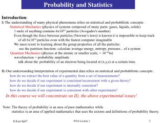
Terminology • Statistic: Science of collecting, analyzing and interpreting data through the application of probability concepts. • Probability: A measure that describes the chance (likelihood) that an event will occur. In simulation applications, probability and statistics are needed to • choose the input distributions of random variables, • generate random variables, • validate the simulation model, • analyze the output. Appendix C – A Refresher on Probability and Statistics
Terminology • Event: Any possible outcome or any set of possible outcomes. • Sample Space: Set of all possible outcomes. • Ex: How is the weather today? • What is the outcome when you toss a coin? • Probability of an Event:Ex: Determine the probability of outcomes when an unfair coin is tossed?Toss the coin several times (say N) under the same conditions.Event A: Head appears Frequency of event A Define Relative frequency of event A Then Appendix C – A Refresher on Probability and Statistics
Probability Basics (cont’d.) • Conditional probability • Knowing that an event F occurred might affect the probability that another event E also occurred • Reduce the effective sample space from S to F, then measure “size” of E relative to its overlap (if any) in F, rather than relative to S • Definition (assuming P(F) 0): • E and F are independent if P(EF) = P(E) P(F) • Implies P(E|F) = P(E) and P(F|E) = P(F), i.e., knowing that one event occurs tells you nothing about the other • If E and F are mutually exclusive, are they independent? Appendix C – A Refresher on Probability and Statistics
Random Variables • One way of quantifying, simplifying events and probabilities • A random variable (RV) is a number whose value is determined by the outcome of an experiment • Technically, a function or mapping from the sample space to the real numbers, but can usually define and work with a RV without going all the way back to the sample space • Think: RV is a number whose value we don’t know for sure but we’ll usually know something about what it can be or is likely to be • Usually denoted as capital letters: X, Y, W1, W2, etc. • Probabilistic behavior described by distribution function Appendix C – A Refresher on Probability and Statistics
Random Variables • Random Var:is a real and single valued function f(E): S R defined on each element E in the sample space S. F( E ) event1 event2 R . . . eventn Thus for each event there is a corresponding random variable Appendix C – A Refresher on Probability and Statistics
Random Variables in Simulation • Ex: In a simulation study how do we decide whether a customer is smoker or not? • Let P( Smoker ) = 0.3 and P( Nonsmoker ) = 0.7 • Generate a random number between [0,1] • If it is < 0.3 smoker • else nonsmoker Appendix C – A Refresher on Probability and Statistics
Discrete vs. Continuous RVs • Two basic “flavors” of RVs, used to represent or model different things • Discrete – can take on only certain separated values • Number of possible values could be finite or infinite • Continuous – can take on any real value in some range • Number of possible values is always infinite • Range could be bounded on both sides, just one side, or neither Appendix C – A Refresher on Probability and Statistics
Discrete Random Variables Probability Mass Function is defined as Ex: Demand of a product, X has the following probability function P(X) 1/3 1/6 X X1 X2 X3 X4 Appendix C – A Refresher on Probability and Statistics
Discrete Random Variables Cumulative distribution function, F(x) is defined as where F(x) is the distribution or cumulative distribution function of X. Ex: F(x) 1 5/6 1/2 1/6 x 1 2 3 4 Appendix C – A Refresher on Probability and Statistics
Expected Value of a Discrete R.V. • Data set has a “center” – the average (mean) • RVs have a “center” – expected value, • What expectation is not: The value of X you “expect” to get! E(X) might not even be among the possible values x1, x2, … • What expectation is: Repeat “the experiment” many times, observe many X1, X2, …, Xn E(X) is what converges to (in a certain sense) as n, where Appendix C – A Refresher on Probability and Statistics
Variances andStandard Deviationof a Discrete R.V. • Data set has measures of “dispersion” – • Sample variance • Sample standard deviation • RVs have corresponding measures • Weighted average of squared deviations of the possiblevalues xi from the mean. • Standard deviation of X is Appendix C – A Refresher on Probability and Statistics
Continuous Distributions • Now let X be a continuous RV • Possibly limited to a range bounded on left or right or both. • No matter how small the range, the number of possible values for X is always (uncountably) infinite • Not sensible to ask about P(X = x) even if x is in the possible range P(X = x) = 0 • Instead, describe behavior of X in terms of its falling between two values! Appendix C – A Refresher on Probability and Statistics
Continuous Distributions (cont’d.) • Probability density function (PDF) is a function f(x) with the following three properties: f(x) 0 for all real values x The total area under f(x) is 1: • Although P(X=x)=0, • Fun facts about PDFs • Observed X’s are denser in regions where f(x) is high • The height of a density, f(x), is not the probability of anything – it can even be > 1 • With continuous RVs, you can be sloppy with weak vs. strong inequalities and endpoints Appendix C – A Refresher on Probability and Statistics
Continuous Random Variables Cumulative distribution function Let I = [a,b] F(x) 1 X Appendix C – A Refresher on Probability and Statistics
Continuous Random Variables • Ex: Lifetime of a laser ray device used to inspect cracks in aircraft wings is given by X, with pdf 1/2 X (years) 2 3 Appendix C – A Refresher on Probability and Statistics
Continuous Expected Values, Variances, and Standard Deviations • Expectation or mean of X is • Roughly, a weighted “continuous” average of possible values for X • Same interpretation as in discrete case: average of a large number (infinite) of observations on the RV X • Variance of X is • Standard deviation of X is Appendix C – A Refresher on Probability and Statistics
Independent RVs • X1 and X2 are independent if their joint CDF factors into the product of their marginal CDFs: • Equivalent to use PMF or PDF instead of CDF • Properties of independent RVs: • They have nothing (linearly) to do with each other • Independence uncorrelated • But not vice versa, unless the RVs have a joint normal distribution • Important in probability – factorization simplifies greatly • Tempting just to assume it whether justified or not • Independence in simulation • Input: Usually assume separate inputs are indep. – valid? • Output: Standard statistics assumes indep. – valid?!?!?!? Appendix C – A Refresher on Probability and Statistics
Sampling • Statistical analysis – estimate or infer something about a population or process based on only a sample from it • Think of a RV with a distribution governing the population • Random sample is a set of independent and identically distributed (IID) observations X1, X2, …, Xn on this RV • In simulation, sampling is making some runs of the model and collecting the output data • Don’t know parameters of population (or distribution) and want to estimate them or infer something about them based on the sample Appendix C – A Refresher on Probability and Statistics
Population parameter Population mean m = E(X) Population variance s2 Population proportion Parameter – need to know whole population Fixed (but unknown) Sample estimate Sample mean Sample variance Sample proportion Sample statistic – can be computed from a sample Varies from one sample to another – is a RV itself, and has a distribution, called the sampling distribution Sampling (cont’d.) Appendix C – A Refresher on Probability and Statistics
Sampling Distributions • Have a statistic, like sample mean or sample variance • Its value will vary from one sample to the next • Some sampling-distribution results • Sample mean If Regardless of distribution of X, • Sample variance s2 E(s2) = s2 • Sample proportion E( ) = p Appendix C – A Refresher on Probability and Statistics
Point Estimation • A sample statistic that estimates (in some sense) a population parameter • Properties • Unbiased: E(estimate) = parameter • Efficient: Var(estimate) is lowest among competing point estimators • Consistent: Var(estimate) decreases (usually to 0) as the sample size increases Appendix C – A Refresher on Probability and Statistics
Confidence Intervals • A point estimator is just a single number, with some uncertainty or variability associated with it • Confidence interval quantifies the likely imprecision in a point estimator • An interval that contains (covers) the unknown population parameter with specified (high) probability 1 – a • Called a 100 (1 – a)% confidence interval for the parameter • Confidence interval for the population mean m: Appendix C – A Refresher on Probability and Statistics
Confidence Intervals in Simulation • Run simulations, get results • View each replication of the simulation as a data point • Random input random output • Form a confidence interval • If you observe the system infinitely many times, 100 (1 – a)% of the time this inerval will contain the true population mean! Appendix C – A Refresher on Probability and Statistics
Hypothesis Tests • Test some assertion about the population or its parameters • Can never determine truth or falsity for sure – only get evidence that points one way or another • Null hypothesis (H0) – what is to be tested • Alternate hypothesis (H1 or HA) – denial of H0 H0: m = 6 vs. H1: m 6 H0: s < 10 vs. H1: s 10 H0: m1 = m2 vs. H1: m1m2 • Develop a decision rule to decide on H0 or H1 based on sample data Appendix C – A Refresher on Probability and Statistics
Errors in Hypothesis Testing Appendix C – A Refresher on Probability and Statistics
p-Values for Hypothesis Tests • Traditional method is “Accept” or Reject H0 • Alternate method – compute p-value of the test • p-value = probability of getting a test result more in favor of H1 than what you got from your sample • Small p (like < 0.01) is convincing evidence against H0 • Large p (like > 0.20) indicates lack of evidence against H0 • Connection to traditional method • If p < a, reject H0 • If pa, do not reject H0 • p-value quantifies confidence about the decision Appendix C – A Refresher on Probability and Statistics
Hypothesis Testing in Simulation • Input side • Specify input distributions to drive the simulation • Collect real-world data on corresponding processes • “Fit” a probability distribution to the observed real-world data • Test H0: the data are well represented by the fitted distribution • Output side • Have two or more “competing” designs modeled • Test H0: all designs perform the same on output, or test H0: one design is better than another Appendix C – A Refresher on Probability and Statistics