Download
1 / 19
250 likes | 1.22k Views
Probability and Statistics. Introduction : I) The u nderstanding of many physical phenomena relies on statistical and probabilistic concepts: Statistical Mechanics (physics of systems composed of many parts: gases, liquids, solids)

E N D
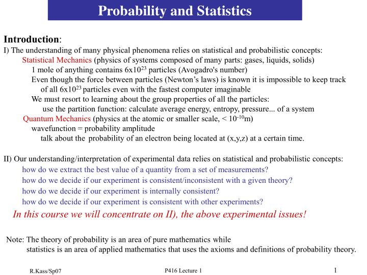
Probability and Statistics Introduction: I)The understanding of many physical phenomena relies on statistical and probabilistic concepts: Statistical Mechanics (physics of systems composed of many parts: gases, liquids, solids) 1 mole of anything contains 6x10²³ particles (Avogadro's number) Even though the force between particles (Newton’s laws) is known it is impossible to keep track of all 6x10²³ particles even with the fastest computer imaginable We must resort to learning about the group properties of all the particles: use the partition function: calculate average energy, entropy, pressure... of a system Quantum Mechanics (physics at the atomic or smaller scale, < 10-10m) wavefunction = probability amplitude talk about the probability of an electron being located at (x,y,z) at a certain time. II) Our understanding/interpretation of experimental data relies on statistical and probabilistic concepts: how do we extract the best value of a quantity from a set of measurements? how do we decide if our experiment is consistent/inconsistent with a given theory? how do we decide if our experiment is internally consistent? how do we decide if our experiment is consistent with other experiments? In this course we will concentrate on II), the above experimental issues! Note: The theory of probability is an area of pure mathematics while statistics is an area of applied mathematics that uses the axioms and definitions of probability theory. P416 Lecture 1
An Example from Particle Physics The understanding and interpretation of all experimental data depend on statistical and probabilistic concepts: “The result of the experiment was inconclusive so we had to use statistics” how do we extract the best value of a quantity from a set of measurements? how do we decide if our experiment is consistent/inconsistent with a given theory? how do we decide if our experiment is internally consistent? how do we decide if our experiment is consistent with other experiments? how do we decide if we have a signal (i.e. evidence for a new particle)? Many of the process involved with detection of particles are statistical in nature: Number of ion pairs created when proton goes through 1 cm of gas Energy lost by an electron going through 1 mm of lead K+n=Q5=dudus Consider the pentaquark from the SPring-8 (LEPS) experiment: signal: 19 events Significance: 4.6s (Assuming gaussian stats the prob. for a 4.6s effect is ~4x10⁻⁶) What are the authors trying to say here? If this bump is accidental, then the accident rate is 1 in 4 million. Or If I repeated the experiment 4 million times I would get a bump this big or bigger. What do the authors want you to think? Since the accident rate is so low it must not be an accident, therefore it is physics! P416 Lecture 1
Sometimes it is not a question of statistical significance! Again, the pentaquark state Q+(1540) gives a great example: Consider the CLAS experiment at JLAB: 2003/4 report a 7.8s effect (~6x10-15 according to MATHEMATICA) 2005 report NO Signal! (better experiment) Pentaquark Reality CLAS 2005 g11 CLAS 2003/2004 What size signal should we expect? Lesson: This is not a statistics issue, but one of experiment design and implementation. P416 Lecture 1
How do we define Probability? Definition of probability by example: l Suppose we have N trials and a specified event occurs r times. example: the trial could be rolling a dice and the event could be rolling a 6. define probability (P) of an event (E) occurring as: P(E) = r/N when N ®¥ examples: six sided dice:P(6) = 1/6 for an honest dice: P(1) = P(2) = P(3) = P(4) =P(5) = P(6) =1/6 coin toss:P(heads) = P(tails) =0.5 P(heads) should approach 0.5 the more times you toss the coin. For a single coin toss we can never get P(heads) = 0.5! u By definition probability (P) is a non-negative real number bounded by 0£ P£1 if P = 0 then the event never occurs if P = 1 then the event always occurs Let A and B be subsets of S then P(A)≥0, P(B)≥0 Events are independent if: P(AÇB) = P(A)P(B) Coin tosses are independent events, the result of the next toss does not depend on previous toss. Events are mutually exclusive (disjoint) if: P(AÇB) = 0 or P(AÈB) = P(A) + P(B) In tossing a coin we either get a head or a tail. Sum (or integral) of all probabilities if they are mutually exclusive must = 1. A= {1,2,3} B={1,3,5} AÇB={1,3} AÈB= {1,2,3,5} Ǻintersection Ⱥ union P416 Lecture 1
lProbability can be a discrete or a continuous variable. Discrete probability: P can have certain values only. examples: tossing a six-sided dice: P(xi) = Pi here xi = 1, 2, 3, 4, 5, 6 and Pi = 1/6 for all xi. tossing a coin: only 2 choices, heads or tails. for both of the above discrete examples (and in general) when we sum over all mutually exclusive possibilities: Continuous probability:P can be any number between 0 and 1. define a “probability density function”, pdf, f(x): with a a continuous variable Probability for x to be in the rangea£ x£b is: Just like the discrete case the sum of all probabilities must equal 1. We say that f(x) is normalized to one. Probability for x to be exactly some number is zero since: NOTATION xi is called a random variable Probability=“area under the curve” Note: in the above example the pdf depends on only 1 variable, x. In general, the pdf can depend on many variables, i.e. f=f(x,y,z,…). In these cases the probability is calculated using from multi-dimensional integration. P416 Lecture 1
lExamples of some common P(x)’s and f(x)’s: Discrete = P(x) Continuous = f(x) binomial uniform, i.e. constant Poisson Gaussian exponential chi square lHow do we describe a probability distribution? u mean, mode, median, and variance u for a normalized continuous distribution, these quantities are defined by: u for a discrete distribution, the mean and variance are defined by: P416 Lecture 1
Remember: Probability is the area under these curves! For many pdfs its integral can not be done in closed form, use a table to calculate probability. Some Continuous Probability Distributions For a Gaussian pdf the mean, mode, and median are all at the same x. For many pdfs the mean, mode, and median are in different places. v=1 ÞCauchy (Breit-Wigner) v=¥ Þgaussian u Chi-square distribution Student t distribution P416 Lecture 1
lCalculation of mean and variance: example: a discrete data set consisting of three numbers: {1, 2, 3} average () is just: Complication: suppose some measurements are more precise than others. Let each measurement xi have a weight wi associated with it then: variance (2) or average squared deviation from the mean is just: is called the standard deviation rewrite the above expression by expanding the summations: Note: The n in the denominator would be n -1 if we determined the average (m) from the data itself. “weighted average” The variance describes the width of the pdf ! This is sometimes written as: <x2>-<x>2 with <>º average of what ever is in the brackets P416 Lecture 1
Using the definition of m from above we have for our example of {1,2,3}: The case where the measurements have different weights is more complicated: Here m is the weighted mean If we calculated m from the data, 2 gets multiplied by a factor n/(n-1). Example: a continuous probability distribution, This “pdf” has two modes! It has same mean and median, but differ from the mode(s). P416 Lecture 1
For continuous probability distributions, the mean, mode, and median are calculated using either integrals or derivatives: u example: Gaussian distribution function, a continuous probability distribution f(x)=sin2x is not a true pdf since it is not normalized! f(x)=(1/p) sin2x is a normalized pdf (c=1/p). In this class you should feel free to use a table of integrals and/or derivatives. P416 Lecture 1
Accuracy and Precision Accuracy: The accuracy of an experiment refers to how close the experimental measurement is to the true value of the quantity being measured. Precision: This refers to how well the experimental result has been determined, without regard to the true value of the quantity being measured. Just because an experiment is precise it does not mean it is accurate!! example: measurements of the neutron lifetime over the years: Steady increase in precision of the neutron lifetime but are any of these measurements accurate? The size of bar reflects the precision of the experiment This figure shows various measurements of the neutron lifetime over the years. P416 Lecture 1
Measurement Errors (or uncertainties) Use results from probability and statistics as a way of calculating how “good” a measurement is. most common quality indicator: relative precision = [uncertainty of measurement]/measurement example: we measure a table to be 10 inches with uncertainty of 1 inch. relative precision = 1/10 = 0.1 or 10% (% relative precision) Uncertainty in measurement is usually square root of variance: s = standard deviation s is usually calculated using the technique of “propagation of errors”. Statistical and Systematic Errors Results from experiments are often presented as: N ± XX ± YY N: value of quantity measured (or determined) by experiment. XX: statistical error, usually assumed to be from a Gaussian distribution. With the assumption of Gaussian statistics we can say (calculate) something about how well our experiment agrees with other experiments and/or theories. Expect ~ 68% chance that the true value is between N - XX and N + XX. YY: systematic error. Hard to estimate, distribution of errors usually not known. examples: mass of proton = 0.9382769 ± 0.0000027 GeV (only statistical error given) mass of W boson = 80.8 ± 1.5 ± 2.4 GeV (both statistical and systematic error given) P416 Lecture 1
What’s the difference between statistical and systematic errors? N ± XX ± YY Statistical errors are “random” in the sense that if we repeat the measurement enough times: XX ®0 as the number of measurements increases Systematic errors, YY, do not® 0 with repetition of the measurements. examples of sources of systematic errors: voltmeter not calibrated properly a ruler not the length we think is (meter stick might really be < meter!) Because of systematic errors, an experimental result can be precise, but not accurate! How do we combine systematic and statistical errors to get one estimate of precision? BIG PROBLEM! two choices: tot = XX + YY add them linearly tot = (XX2 + YY2)1/2 add them in quadrature Some other ways of quoting experimental results lower limit: “the mass of particle X is > 100 GeV” upper limit: “the mass of particle X is < 100 GeV” asymmetric errors: mass of particle P416 Lecture 1
The relationships and results from set theory are essential to the understanding of probability. Below are some definitions and examples that illustrate the connection between set theory, probability and statistics. Probability, Set Theory and Stuff We define an experiment as a process that generates “observations” and a sample space (S) as the set of all possible outcomes from the experiment: simple event: only one possible outcome compound event: more than one outcome As an example of simple and compound events consider particles (e.g. protons, neutrons) made of u (“up”), d (“down”), and s (“strange”) quarks. The u quark has electric charge (Q) =2/3|e| (e=charge of electron) while the d and s quarks have charge =-1/3|e|. Let the experiment be the ways we combine 3 quarks to make a Q=0, 1, or 2 state. Event A: Q=0 {ssu, ddu, sdu} note: a neutron is a ddu state Event B: Q=1{suu, duu} note: a proton is a duu state Event C: Q=2 {uuu} For this example events A and B are compound while event C is simple. The following definitions from set theory are used all the time in the discussion of probability. Let A and B be events in a sample space S. Union: The union of A & B (AÈB) is the event consisting of all outcomes in A or B. Intersection: The intersection of A & B (AÇB) is the event consisting of all outcomes in A and B. Complement: The complement of A (A´) is the set of outcomes in S not contained in A. Mutually exclusive: If A & B have no outcomes in common they are mutually exclusive. P416 Lecture 1
Returning to our example of particles containing 3 quarks (“baryons”): The event consisting of charged particles with Q=1,2 is the union of B and C: BÈC The events A, B, C are mutually exclusive since they do not have any particles in common. Probability, Set Theory and Stuff A common and useful way to visualize union, intersection, and mutually exclusive is to use a Venn diagram of sets A and B defined in space S: B B A A A B B S A S S S AÇB: intersection of A&B AÈB: union of A&B Venn diagram of A&B A & B mutually exclusive The axioms of probabilities (P): a) For any event A, P(A)≥0. (no negative probabilities allowed) b) P(S)=1. c) If A1, A2, ….An is a collection of mutually exclusive events then: (the collection can be infinite (n=∞)) From the above axioms we can prove the following useful propositions: a) For any event A: P(A)=1-P(A´) b) If A & B are mutually exclusive then P(AÇB)=0 c) For any two events A & B: P(AÈB)=P(A)+P(B)-P(AÇB) items b, c are “obvious” from their Venn diagrams P416 Lecture 1
Example: Everyone likes pizza. Assume the probability of having pizza for lunch is 40%, the probability of having pizza for dinner is 70%, and the probability of having pizza for lunch and dinner is 30%. Also, this person always skips breakfast. We can recast this example using: P(A)= probability of having pizza for lunch =40% P(B)= probability of having pizza for dinner = 70% P(AÇB)=30% (pizza for lunch and dinner) 1) What is the probability that pizza is eaten at least once a day? The key words are “at least once”, this means we want the union of A & B P(AÈB)=P(A)+P(B)-P(AÇB) = .7+.4-.3 =0.8 2) What is the probability that pizza is not eaten on a given day? Not eating pizza (Z´) is the complement of eating pizza (Z) so P(Z)+P(Z´)=1 P(Z´)=1-P(Z) =1-0.8 = 0.2 3) What is the probability that pizza is only eaten once a day? This can be visualized by looking at the Venn diagram and realizing we need to exclude the overlap (intersection) region. P(AÈB)-P(AÇB) = 0.8-0.3 =0.5 Probability, Set Theory and Stuff prop. c) prop. a) pizza for lunch The non-overlapping blue area is pizza for lunch, no pizza for dinner. The non-overlapping red area is pizza for dinner, no pizza for lunch. pizza for dinner P416 Lecture 1
Conditional Probability Frequently we must calculate a probability assuming something else has occurred. This is called conditional probability. Here’s an example of conditional probability: Suppose a day of the week is chosen at random. The probability the day is Thursday is 1/7. P(Thursday)=1/7 Suppose we also know the day is a weekday. Now the probability is conditional, =1/5. P(Thursday|weekday)=1/5 the notation is: probability of it being Thursday given that it is a weekday Formally, we define the conditional probability of A given B has occurred as: P(A|B)=P(AÇB)/P(B) We can use this definition to calculate the intersection of A and B: P(AÇB)=P(A|B)P(B) For the case where the Ai’s are both mutually exclusive and exhaustive we have: For our example let B=the day is a Thursday, A1= weekday, A2=weekend, then: P(Thursday)=P(thursday|weekday)P(weekday)+P(Thursday|weekend)P(weekend) P(Thursday)=(1/5)(5/7)+(0)(2/7)=1/7 P416 Lecture 1
Bayes’s Theorem relates conditional probabilities. It is widely used in many areas of the physical and social sciences. Bayes’s Theorem Let A1, A2,..Ai be a collection of mutually exclusive and exhaustive events with P(Ai)>0 for all i. Then for any other event B with P(B)>0 we have: We call: P(Aj) the aprori probability of Aj occurring P(Aj|B) the posterior probability that Aj will occur given that B has occurred P(B|Aj) the likelihood Independence has a special meaning in probability: Events A and B are said to be independent if P(A|B)=P(A) Using the definition of conditional probability A and B are independent iff: P(AÇB)=P(A)P(B) P416 Lecture 1
While Bayes’s theorem is very useful in physics, perhaps the best illustration of its use is in medical statistics, especially drug testing. Assume a certain drug test: gives a positive result 97% of the time when the drug is present: P(positive test|drug present)=0.97 gives a positive result 0.4% of the time if the drug is not present (“false positive”) P(positive test|drug not present)=0.004 Let’s assume that the drug is present in 0.5% of the population (1 out of 200 people). P(drug present)=0.005 P(drug not present)=1-P(drug present)=0.995 What is the probability that the drug is not present and you have a positive test? P(drug is not present|positive test)=???? Bayes’s Theorem gives: Example of Bayes’s Theorem Thus there is a 45% chance that the test comes back positive even if you are drug free! The real life consequence of this large probability is that drug tests are often administered twice! P416 Lecture 1