Download
1 / 43
470 likes | 635 Views
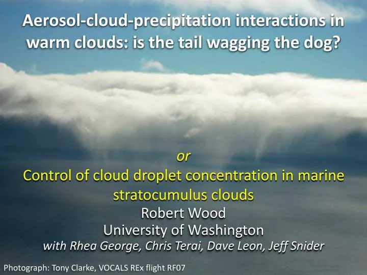
Aerosol-cloud-precipitation interactions in warm clouds: is the tail wagging the dog?. or Control of cloud droplet concentration in marine stratocumulus clouds. Robert Wood University of Washington with Rhea George, Chris Terai , Dave Leon, Jeff Snider.

E N D
Aerosol-cloud-precipitation interactions in warm clouds: is the tail wagging the dog? or Control of cloud droplet concentration in marine stratocumulus clouds Robert Wood University of Washington with Rhea George, Chris Terai, Dave Leon, Jeff Snider Photograph: Tony Clarke, VOCALS REx flight RF07
Radiative impact of cloud droplet concentration variations Satellite-derived cloud droplet concentration Nd albedo enhancement (fractional) low level wind George and Wood, Atmos. Chem. Phys., 2010
“Background” cloud droplet concentration critical for determining aerosol indirect effects LAND OCEAN A ln(Nperturbed/Nunpertubed) Low Nd background strong Twomey effect High Nd background weaker Twomey effect Quaas et al., AEROCOM indirect effects intercomparison, Atmos. Chem. Phys., 2009
Aerosol (D>0.1 mm) vs cloud droplet concentration (VOCALS, SE Pacific) 1:1 line see also... Twomey and Warner (1967) Martin et al. (1994)
Extreme coupling between drizzle and CCN • Southeast Pacific • Drizzle causes cloud morphological transitions • Depletes aerosols Wood et al. (J. Geophys. Res., 2008)
MODIS-estimated mean cloud droplet concentrationNd Can we explain these patterns? • Use method of Boers and Mitchell (1996), applied by Bennartz (2007) • Screen to remove heterogeneous clouds by insisting on CFliq>0.6 in daily L3
Prevalence of drizzle from low clouds DAY NIGHT Leon et al., J. Geophys. Res. (2008) Drizzle occurrence = fraction of low clouds (1-4 km tops) for which Zmax> -15 dBZ
Simple CCN budget in the MBL Model accounts for: • Entrainment • Surface production (sea-salt) • Coalescence scavenging • Dry deposition Model does not account for: • New particle formation – significance still too uncertain to include • Advection – more later
Production terms in CCN budget Entrainment rate FT Aerosol concentration MBL depth Sea-salt parameterization-dependent constant Wind speed at 10 m We use Clarke et al. (J. Geophys. Res., 2007) at 0.4% supersaturation to represent an upper limit
Sea-spray flux parameterizations u10=8 m s-1 Courtesy of Ernie Lewis, Brookhaven National Laboratory
Loss terms in CCN budget: (1) Coalescence scavenging Constant Precip. rate at cloud base cloud thickness MBL depth Comparison against results from stochastic collection equation (SCE) applied to observed size distribution Wood, J. Geophys. Res., 2006
Loss terms in CCN budget: (2) Dry deposition Deposition velocity wdep= 0.002 to 0.03 cm s-1 (Georgi 1988) K = 2.25 m2kg-1 (Wood 2006) For PCB = > 0.1 mm day-1and h = 300 m = 3 to 30 For precip rates > 0.1 mm day-1, coalescence scavenging dominates
October-November 2008 SE Pacific
MODIS-estimated cloud droplet concentration Nd, VOCALS Regional Experiment • Data from Oct-Nov 2008 • Sampling along 20oS across strong microphysical gradient
Free tropospheric CCN source Weber and McMurry (FT, Hawaii) Continentally- influenced FT Remote “background” FT Data from VOCALS (Jeff Snider) S=0.9% 0.5 0.25 0.1 S = 0.9% S = 0.25%
Conceptual model of background FT aerosol Clarke et al. (J. Geophys. Res. 1998)
Self-preserving aerosol size distributions • after Friedlander, explored by Raes: Fixed supersaturation: 0.8% 0.4% 0.2% Variable supersat. 0.3 0.2% Kaufman and Tanre (Nature 1994) Raes et al., J. Geophys. Res. (1995)
Observed MBL aerosol dry size distributions (SE Pacific) 0.08 mm 0.06 Tomlinson et al., J. Geophys. Res. (2007)
Precipitation over the VOCALS region • CloudSatAttenuation and Z-R methods • VOCALS Wyoming Cloud Radar and in-situ cloud probes Significant drizzle at 85oW Very little drizzle near coast WCR data courtesy Dave Leon
Predicted and observed Nd, VOCALS • Model increase in Ndtoward coast is related to reduced drizzleand explains the majority of the observed increase • Very close to the coast (<5o) an additional CCN source is required • Even at the heart of the Sc sheet (80oW) coalescence scavenging halves the Nd • Results insensitive to sea-salt flux parameterization 17.5-22.5oS
Predicted and observed Nd • Monthly climatological means (2000-2009 for MODIS, 2006-2009 for CloudSat) • Derive mean for locations where there are >3 months for which there is: • (1) positive large scale div. • (2) mean cloud top height <4 km • (3) MODIS liquid cloud fraction > 0.4 • Use 2C-PRECIP-COLUMN and Z-R where 2C-PRECIP-COLUMN missing
Predicted and observed Nd- histograms Minimum values imposed in GCMs
Mean precipitation rate (CloudSat, 2C-PRECIP-COLUMN, Stratocumulus regions)
Reduction of Nd from precipitation sink • Precipitation from midlatitude low clouds reduces Nd by a factor of 5 • In coastal subtropical Sc regions, precip sink is weak 0 10 20 50 100 150 200 300 500 1000 2000 %
Precipitation closure from Brenguier and Wood (2009) • Precipitation rate dependent upon: • cloud macrophysicalproperties (e.g. thickness, LWP); • microphysical properties (e.g. droplet conc., CCN) precipitation rate at cloud base [mm/day]
Conclusions • Simple CCN budget model, constrained with precipitation rate estimates from CloudSat predicts MODIS-observed cloud droplet concentrations in regions of persistent low level clouds with some skill. • Significant fraction of the variability in Nd across regions of extensive low clouds is likely related to precipitation sinks rather than source variability => there is a tail wagging part of the dog! • It may be difficult to separate the chicken from the egg in correlative studies suggesting inverse dependence of precipitation rate on cloud droplet concentration
A proposal • A limited area perturbation experiment to critically test hypotheses related to aerosol indirect effects • Cost $30M
Precipitation susceptibility • Construct from Feingold and Siebert (2009) can be used to examine aerosol influences on precipitation in both models and observations S = -(dlnRCB/dlnNa)LWP,h • S decreases strongly with cloud thickness • Consistent with increasing importance of accretion in thicker clouds • Consistent with results from A-Train (Kubar et al. 2009, Wood et al. 2009) Data from stratocumulus over the SE Pacific, Terai and Wood (Geophys. Res. Lett., 2011)
Effect of variable supersaturation Constant s • Kaufman and Tanre 1994 Variable s
Range of observed and modeled CCN/droplet concentration in Baker and Charlson “drizzlepause” region where loss rates from drizzle are maximal • Baker and Charlson source rates Baker and Charlson, Nature (1990)
Timescales to relax for N Entrainment: Surface: tsfc Precip: zi/(hKPCB) = 8x10^5/(3*2.25) = 1 day for PCB=1 mm day-1 tdepzi/wdep - typically 30 days
Can dry deposition compete with coalescence scavenging? wdep= 0.002 to 0.03 cm s-1 (Georgi 1988) K = 2.25 m2kg-1 (Wood 2006) For PCB = > 0.1 mm day-1and h = 300 m = 3 to 30 For precip rates > 0.1 mm day-1, coalescence scavenging dominates
Examine MODIS Nd imagery – fingerprinting of entrainment sources vs MBL sources.
Cloud droplet concentrations in marine stratiform low cloud over ocean The view from MODIS ....how can we explain this distribution? Nd [cm-3] Latham et al., Phil. Trans. Roy. Soc. (2011)
Baker and Charlson model 200 100 0 -100 -200 -300 -400 -500 • CCN/cloud droplet concentration budget with sources (specified) and sinks due to drizzle (for weak source, i.e. low CCN conc.) and aerosol coagulation (strong source, i.e. high CCN conc.) • Stable regimes generated at point A (drizzle) and B (coagulation) • Observed marine CCN/Nd values actually fall in unstable regime! observations CCN loss rate [cm-3 day-1] 10 100 1000 CCN concentration [cm-3] Baker and Charlson, Nature (1990)
Baker and Charlson model 200 100 0 -100 -200 -300 -400 -500 • Stable region A exists because CCN loss rates due to drizzle increase strongly with CCN concentration • In the real world this is probably not the case, and loss rates are constant with CCN conc. • However, the idea of a simple CCN budget model is alluring observations CCN loss rate [cm-3 day-1] 10 100 1000 CCN concentration [cm-3] Baker and Charlson, Nature (1990)