Download
1 / 51
510 likes | 692 Views
Black Box. Op { X , Z }. X. Y. Z. Bündel von Leitungen. Signalklassifizierung. x(t). x(k). t. k. x(t). x(k). T A. t. k. T A. Zustandstabelle. x(t). x(t). x bin. ES. 1. 0. t. t. t. Zuordnung. x bin. T O. 1. T U. 0. t. Blockschaltbild. x. y. f(x). x. y. x.

E N D
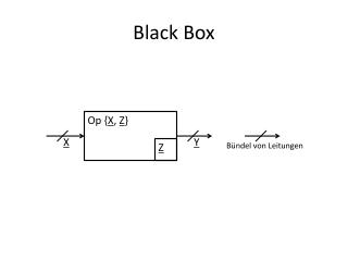
Black Box Op {X, Z} X Y Z Bündel von Leitungen
Signalklassifizierung x(t) x(k) t k x(t) x(k) TA t k TA
Zustandstabelle x(t) x(t) xbin ES 1 0 t t t Zuordnung xbin TO 1 TU 0 t
Blockschaltbild x y f(x) x y x y f(x) f(x)
BDD f Wurzelknoten root-node V1 x0 0 1 V2 V3 innere Knoten internalnodes x1 0 1 0 1 V4 V5 V6 V7 x2 0 1 0 1 0 1 0 1 Endknoten terminal nodes (enthalten f-Werte) 0 0 1 0 0 1 1 1
BDD f f V1 V1 x0 0 1 0 1 V2 V3 V2 V3 x1 0 1 0 1 0 1 0 1 V4 V5 V6 V7 V5 V6 x2 0 1 0 1 0 1 0 1 1 0 1 0 0 1 0 1
Verhaltensmodell a b y1=f(x) x c z=h*(y)=h(x) y2=g(x)
Abbildungsprodukt a z=h(x) b c
Kontaktschaltungen + + + + + + r f2=a f1 f2 f3 f4 R RK a AK RK a
Gatterschaltungen + Tp p-leitend 1 a a f2=a n-leitend high low Tp Tn f2=a low high high Tn low
Kontaktschaltungen + + f5 f6 a a b b
Gatterschaltungen + + a & f5=ab b a b p p a 1 f6=ab fNAND b fNAND a a a & fNAND b n b b n
Analyse und Vereinfachung + + a b a b c a c f b f
XOR und XAND a =1 b a = f~ b
Orthogonalität 011 111 001 101 010 110 x2 x1 000 100 x0
MUX8to1 a=1 a=0 a=1 a=0 a=1 a=0 a=1 a=0 b=1 b=0 b=1 b=0 c=1 c=0 f(0,0,0) MUX 8-to-1 f(c) … f(1,1,1) a b c
Transformation Disjunktive Form D(f) Konjunktive Form K(f) BF, KP, TVL Orthogonalisierung Antivalenzform A(f) Äquivalenzform E(f)
Gatter- und Zweigschaltung a & 1 b + f c f a c b
Analyse des Verhaltens a v1 & b 1 a f‘(x) =1 a b & v2 b
Analyseprinzip a g2 g1 & & & & f(x) b g3
Prinzip x1 ? ? x2 ? f(x) … x2 xk ? 1., 2. Stufe 0. Stufe (Negation)
Beispiel c c & 1 & & 1 1 1 & a a & f & f 1 f 1 f b b a a a a a a a a a a & & 1 1 c c 1 & 1 1 & & b b b b & 1 c c a a a a f f f f 1 1 & & b b c c c c c c c c c c
Einfache Synthese a1 a1 & & & … ai ai f(x) f(x) ai+1 & … ai+1 & an … an a1 & & & … f(x) & & … an
Multiplexer MUX 4-to-1 f1,1 11 MUX 2-to-1 f(a=1) 1 f1,0 10 f(x) f(x) f0,1 01 f(a=0) 0 f0,0 00 a a b c MUX 4-to-1 1 11 d 10 f(x) 1 01 c =1 00 d d a b
Statische Nebenbedingungen a b a & & d fopt b & c
Praktische Erfahrung x(t) y(t) e a z s e/a s 1s 1s1 e/a 1s2 s e/a … e/a 1sn
zeitliches Verhalten e(0)/a(0) e(1)/a(1) … s(0) s(1) s(1) s(n) Anfangs- zustand
Moore und Mealy e s a δ δ λ s s e s a λ
Automatenmodelle β /0 e/a s 1s α/1 1 2 Ursache Wirkung T4 – Zyklus (Länge 4) für α β/0 β /1 α/1 α/1 α/1 3 4 β /0 β /0 5 α/0
Beispiel x/y z 1z y x z1z2 1z11z2 Moore Automat
Beispiel y=1 0 01 11 x=0 z2 1 01 0 z1 z1z2 x=1 00 10 x=1 x=0 1 0
Automatengraph des FF F0 Q 0 1 F0 F1 F1
Struktur von FF-Schaltwerken 1z1 z1 λ kombi-natorisches Bündel kombinatorisches Funktionenbündel für 1z = f(x, z) FF1 x y z … FFk zk 1zk C = Takt an jeden FF C
Master-Slave-Technik x Master FF Slave FF Q
FF-Schema E1 Q E2 … Ei1 & … Eik … Q S T Q CLK J S CLK J Q K CLK R K R
RS-FF 0 1 S S R 1 0 1 Q 0 1 R 1 Q R S 0 1 1 0
JK-FF J J & K (=R) 1 Q 0 1 K C Q 1 K & J (=S)
JR-FF und SK-FF SK JR RJ SK S 0 1 R S 0 1 R
D-FF und T-FF D T D T T D Q 0 0 1 1 D C D T T Q C
RST-FF und L-FF ST 0 1 ST L RT L RT & 0 1 1 R Q & L
Synthese C C(t) 1 1 t t 0 0 Q(t)dyn 1 t 0
Entwurfsbeispiel 1 Zwischenfunktion 1z bilden bei Taktflanke 1 1 D a a z 1 D Q z b b 1 C
Entwurfsbeispiel 1 b D Q z a & R Q z b a b a & & C b C V a & & S b 1. Möglichkeit 2. Möglichkeit
Entwurfsbeispiel 1 & & a a b z T Q z & b C
Entwurfsbeispiel 2 S z1z0 0 00 2 10 1 01 - 11 unbekannter Zustand x x x x x x
Entwurfsbeispiel 2 R1 R0 z1=y1 z0=y0 R Q R Q x x z1 x z1 z0 z0 x & & & & C C z0 S S & S1 & S0 z1
Veranschaulichung des Verhaltens x, y z 1z Kante Phase (x, z, 1z, y) Ursache Wirkung
Beispiel D1 z1=D2 z2=J3 z3=y =1 D Q D Q J Q x C C C V2 K3 V K
Automatengraph 011 111 z1z2z3 001 101 010 110 x=0 000 100
Speichertechnische Realisierung Memory y(t-1) (1z, y) x Adresse z Takt an jedes Register FF-Register 0/0 10 11 1/1 z1z0 x/y 0/0 1/1 1/0 00 01 0/1