Download
1 / 31
310 likes | 512 Views
FROM ANALOG TO DIGITAL DOMAIN. Dr.M.A.Kashem Asst. Professor, CSE,DUET. TOPICS. 1. Analog vs. digital: why, what & how 2. Digital system example 3. Sampling & aliasing 4. ADCs: performance & choice 5. Digital data formats. Analog. Digital.

E N D
FROM ANALOG TO DIGITAL DOMAIN Dr.M.A.Kashem Asst. Professor, CSE,DUET
TOPICS 1. Analog vs. digital: why, what & how 2. Digital system example 3. Sampling & aliasing 4. ADCs: performance & choice 5. Digital data formats M. E. Angoletta - DISP2003 - From analog to digital domain 2 / 30
Analog Digital Discrete function Vk of discrete sampling variable tk, with k = integer: Vk = V(tk). Continuous function V of continuous variable t (time, space etc) : V(t). Uniform (periodic) sampling. Sampling frequency fS = 1/ tS Analog & digital signals M. E. Angoletta - DISP2003 - From analog to digital domain 3 / 30
Limitations Advantages • A/D & signal processors speed: wide-band signals still difficult to treat (real-time systems). • Finite word-length effect. • Obsolescence (analog electronics has it, too!). • More flexible. • Often easier system upgrade. • Data easily stored. • Better control over accuracy requirements. • Reproducibility. Digital vs analog proc’ing Digital Signal Processing (DSPing) M. E. Angoletta - DISP2003 - From analog to digital domain 4 / 30
Predicting a system’s output. • Implementing a certain processing task. • Studying a certain signal. Applications • General purpose processors (GPP), -controllers. • Digital Signal Processors (DSP). • Programmable logic ( PLD, FPGA ). Hardware Fast Faster real-time DSPing • Programming languages: Pascal, C / C++ ... • “High level” languages: Matlab, Mathcad, Mathematica… • Dedicated tools (ex: filter design s/w packages). Software DSPing: aim & tools M. E. Angoletta - DISP2003 - From analog to digital domain 5 / 30
General scheme ANALOG DOMAIN FilterAntialiasing FilterAntialiasing Sometimes steps missing - Filter + A/D (ex: economics); - D/A + filter (ex: digital output wanted). A/D A/D DIGITAL DOMAIN Digital Processing Digital Processing D/A ANALOG DOMAIN Topics of this lecture. FilterReconstruction Digital system example M. E. Angoletta - DISP2003 - From analog to digital domain 6 / 30
ANALOG INPUT Antialiasing Filter 1 2 3 A/D Digital Processing • Digital format. What to use for processing? See slide “DSPing aim & tools” DIGITAL OUTPUT Digital system implementation KEY DECISION POINTS: Analysis bandwidth, Dynamic range •Sampling rate. • Pass / stop bands. • No. of bits. Parameters. M. E. Angoletta - DISP2003 - From analog to digital domain 7 / 30
1 * Ex: train wheels in a movie. 25 frames (=samples) per second. Train starts wheels ‘go’ clockwise. Train accelerates wheels ‘go’ counter-clockwise. *Sampling: independent variable (ex: time) continuous discrete. Quantisation: dependent variable (ex: voltage) continuous discrete. Here we’ll talk about uniform sampling. Sampling How fast must we sample a continuous signal to preserve its info content? Why? Frequency misidentification due to low sampling frequency. M. E. Angoletta - DISP2003 - From analog to digital domain 8 / 30
1 __ s(t) = sin(2f0t) s(t) @ fS f0 = 1 Hz, fS = 3 Hz __ s1(t) = sin(8f0t) __ s2(t) = sin(14f0t) s(t) @ fS represents exactly all sine-waves sk(t) defined by: sk (t) = sin( 2 (f0 + k fS) t ) , k Sampling - 2 M. E. Angoletta - DISP2003 - From analog to digital domain 9 / 30
1 Example Condition on fS? F1 F2 F3 fS > 300 Hz F1=25 Hz, F2 = 150 Hz, F3 = 50 Hz fMAX The sampling theorem A signal s(t) with maximum frequency fMAX can be recovered if sampled at frequency fS > 2 fMAX . Theo* *Multiple proposers: Whittaker(s), Nyquist, Shannon, Kotel’nikov. Naming gets confusing ! Nyquist frequency (rate) fN = 2 fMAXor fMAXor fS,MINor fS,MIN/2 M. E. Angoletta - DISP2003 - From analog to digital domain 10 / 30
1 Example Ear + brain act as frequency analyser: audio spectrum split into many narrow bands low-power sounds detected out of loud background. • Bandwidth: indicates rate of change of a signal. High bandwidth signal changes fast. BOOM ! minus 50 Hz ?? Frequency domain (hints) • Time & frequency: two complementary signal descriptions. Signals seen as “projected’ onto time or frequency domains. Warning: formal description makes use of “negative” frequencies ! M. E. Angoletta - DISP2003 - From analog to digital domain 11 / 30
1 (a)Band-limited signal: frequencies in [-B, B] (fMAX = B). (a) (b) (b)Time sampling frequency repetition. fS > 2 B no aliasing. (c) (c)fS 2 B aliasing ! Aliasing: signal ambiguity in frequency domain Sampling low-pass signals M. E. Angoletta - DISP2003 - From analog to digital domain 12 / 30
1 (a) (a),(b)Out-of-band noise can aliase into band of interest. Filter it before! (c)Antialiasing filter (b) • Passband: depends on bandwidth of interest. • Attenuation AMIN : depends on • ADC resolution ( number of bits N). • AMIN, dB ~ 6.02 N + 1.76 • Out-of-band noise magnitude. • Other parameters: ripple, stopband frequency... (c) Antialiasing filter M. E. Angoletta - DISP2003 - From analog to digital domain 13 / 30
1 m , selected so that fS > 2B Example Advantages • Slower ADCs / electronics needed. • Simpler antialiasing filters. fC = 20 MHz, B = 5MHz Without under-sampling fS > 40 MHz. With under-sampling fS = 22.5 MHz (m=1); = 17.5 MHz (m=2); = 11.66 MHz (m=3). Under-sampling (hints) Using spectral replications to reduce sampling frequency fS req’ments. M. E. Angoletta - DISP2003 - From analog to digital domain 14 / 30
1 Oversampling : sampling at frequencies fS >> 2 fMAX . Over-sampling & averaging may improve ADC resolution ( i.e. SNR, see ) fOS = over-sampling frequency, w = additional bits required. 2 fOS = 4w· fS Each additional bit implies over-sampling by a factor of four. Caveat • It works for: • white noise with amplitude sufficient to change the input signal randomly from sample to sample by at least LSB. • Input that can take all values between two ADC bits. Over-sampling (hints) M. E. Angoletta - DISP2003 - From analog to digital domain 15 / 30
2 Different applications have different needs. • Number of bits N (~resolution) • Data throughput (~speed) • Signal-to-noise ratio (SNR) • Signal-to-noise-&-distortion rate (SINAD) • Effective Number of Bits (ENOB) • Spurious-free dynamic range (SFDR) • Integral non-linearity (INL) • Differential non-linearity (DNL) • … Radar systems Static distortion Communication Dynamic distortion Imaging / video NB: Definitions may be slightly manufacturer-dependent! (Some) ADC parameters M. E. Angoletta - DISP2003 - From analog to digital domain 16 / 30
2 Continuous input signal digitized into 2N levels. Uniform, bipolar transfer function (N=3) Quantisation step q = V FSR 2N Ex: VFSR = 1V , N = 12 q = 244.1 V Voltage ( = q) Scale factor (= 1 / 2N ) Percentage (= 100 / 2N ) LSB Quantisation error ADC - Number of bits N M. E. Angoletta - DISP2003 - From analog to digital domain 17 / 30
2 • Quantisation Error eq in [-0.5 q, +0.5 q]. • eq limits ability to resolve small signal. • Higher resolution means lower eq. QE for N = 12 VFS = 1 ADC - Quantisation error M. E. Angoletta - DISP2003 - From analog to digital domain 18 / 30
2 Assumptions (1) • Ideal ADC: only quantisation erroreq (p(e) constant, no stuck bits…) • eq uncorrelated with signal. • ADC performance constant in time. Also called SQNR (signal-to-quantisation-noise ratio) Input(t) = ½ VFSR sin(t). (sampling frequency fS = 2 fMAX) SNR of ideal ADC M. E. Angoletta - DISP2003 - From analog to digital domain 19 / 30
2 One additional bit SNR increased by 6 dB Real SNR lower because: • Real signals have noise. • Forcing input to full scale unwise. • Real ADCs have additional noise (aperture jitter, non-linearities etc). SNR of ideal ADC - 2 Substituting in (1) : (2) Actually (2) needs correction factor depending on ratio between sampling freq & Nyquist freq. Processing gain due to oversampling. M. E. Angoletta - DISP2003 - From analog to digital domain 20 / 30
2 SNR and SINAD often confused in specs. ENOB : N from (2) when setting SNR ideal = SINAD, i.e. ENOB = (SINAD – 1.76 dB) / 6.02. Actual number of bit available to an equivalent ideal ADC Example 12-bit ADC chip, 68 dB SINAD in specs ~ 11-bit ideal ADC. Real ADCs: parameters SNR: (sine_in RMS)/(ADC out_noise RMS), with out_noise = output - (DC + first 5 input harmonics) output components. SINAD: (sine_in RMS)/(ADC out_noise_2 RMS), with out_noise_2 = output - (DC output component). M. E. Angoletta - DISP2003 - From analog to digital domain 21 / 30
2 * High resolution (bit #) - Higher cost & dissipation. - Tailored onto DSP word width. *DIFFICULT area moves down & right every year. Rule of thumb: 1 bit improvement every 3 years. High speed - Large amount of data to store/analyse. - Lower accuracy & input impedance. 2 Oversampling & averaging (see ). Dithering( = adding small random noise before quantisation). may increase SNR. ADC selection dilemma Speed & resolution: a tradeoff. M. E. Angoletta - DISP2003 - From analog to digital domain 22 / 30
3 Integer part Fractional part Early computers (ex: ENIAC) mainly base-10 machines. Mostly turned binary in the ’50s. a) less complex arithmetic h/w; Benefits b) less storage space needed; c) simpler error analysis. Digital data formats Positional number system with baseb: [ .. a2 a1 a0.a-1 a-2 .. ]b = .. + a2 b2 + a1 b1 + a0 b0 + a-1 b-1 + a-2 b-2+ .. Important bases: 10 (decimal), 2 (binary), 8 (octal), 16 (hexadecimal). M. E. Angoletta - DISP2003 - From analog to digital domain 23 / 30
3 Increasing number of applications requires decimal arithmetic. Ex: Banking, Financial Analysis. • Common decimal fractional numbers only approximated by binary numbers. Ex: 0.1 infinite recurring binary fraction. • Non-integer decimal arithmetic software emulation available but often too slow. IEEE 754,1985: binary floating point arithmetic standard specified IEEE 854,1987: standard expanded to include decimal arithmetic. Decimal arithmetic BUT M. E. Angoletta - DISP2003 - From analog to digital domain 24 / 30
3 Ex: 3-bit formats 15 14 ... 0 Unsigned integer Offset-Binary Sign-Magnitude Two’s complement 7111 4111 3011 3 011 6110 3110 2010 2010 MSB LSB 5101 2101 1001 1001 4100 1100 0000 0000 Fractional point (DSPs) 3011 0011 0100 -1111 2010 -1010 -1101 -2110 1001 -2001 -2110 -3101 Sign bit 0000 -3000 -3111 -4100 Decimal equivalent Binary representation Fixed-point binary Represent integer or fractional binary numbers. NB: Constant gap between numbers. M. E. Angoletta - DISP2003 - From analog to digital domain 25 / 30
3 Wide variety of floating point hardware in ‘60s and ‘70s, different ranges, precision and rounded arithmetic. William Kahan: “Reliable portable software was becoming more expensive to develop than anyone but AT&T and the Pentagon could afford”. IEEE 754 standard Definition of IEEE 754 standard between 1977 and 1985. De facto standard before 1985 ! Formats & methods for binary floating-point arithmetic. Note: NOT the easiest h/w choice! Floating-point binary PROBLEM M. E. Angoletta - DISP2003 - From analog to digital domain 26 / 30
3 31 30 23 22 0 Precision e s f MSB LSB Single (32 bits) Double (64 bits) Double-extended ( 80 bits) e = exponent, offset binary, -126 < e < 127 s = sign, 0 = pos, 1 = neg f = fractional part, sign-magnitude + hidden bit Single precision range Max = 3.4 · 1038 Min = 1.175 · 10-38 Coded number x = (-1)s· 2e · 1.f NB: Variable gap between numbers. Large numbers large gaps; small numbers small gaps. Floating-point binary - 2 IEEE 754 standard M. E. Angoletta - DISP2003 - From analog to digital domain 27 / 30
3 Overflow : arises when arithmetic operation result has one too many bits to be represented in a certain format. largest value smallest value Fixed point ~ 180 dB Floating point ~1500 dB Dynamic rangedB= 20 log10 High dynamic range wide data set representation with no overflow. NB: Different applications have different needs. Ex: telecomms: 50 dB; HiFi audio: 90 dB. Finite word-length effects M. E. Angoletta - DISP2003 - From analog to digital domain 28 / 30
3 Round-off: error caused by rounding math calculation result to nearest quantisation level. Example Big concern for real numbers. 0.1 not exactly represented (falls between two floating point numbers). Finite word-length effects - 2 • For integers within ±16.8 million range: single-precision floating point gives no round-off error. • Outside that range, integers are missing: gaps between consecutive floating point numbers are larger than integers. Round-off error estimate: Relative error = (floating - actual value)/actual value (depends on base). The smaller the base, the tighter the error estimate. M. E. Angoletta - DISP2003 - From analog to digital domain 29 / 30
References Papers • On bandwidth, David Slepian, IEEE Proceedings, Vol. 64, No 3, pp 291 - 300. • The Shannon sampling theorem - Its various extensions and applications: a tutorial review, A. J. Jerri, IEEE Proceedings, Vol. 65, no 11, pp 1565 – 1598. • What every computer scientist should know about floating-point arithmetic, David Goldberg. • IEEE Standard for radix-independent floating-point arithmetic, ANSI/IEEE Std 854-1987. Books • Understanding digital signal processing, R. G. Lyons, Addison-Wesley Publishing, 1996. • The scientist and engineer’s guide to digital signal processing, S. W. Smith, at http://www.dspguide.com. • Discrete-time signal processing, A. V. Oppeheim & R. W. Schafer, Prentice Hall, 1999. M. E. Angoletta - DISP2003 - From analog to digital domain 30 / 30
COFFEE BREAK Coffee in room #13 Be back in ~15 minutes M. E. Angoletta - DISP2003 - From analog to digital domain 31 / 30