Download
1 / 37
370 likes | 519 Views
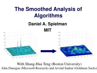
Learning and smoothed analysis. Alex Samorodnitsky* Hebrew University Jerusalem. Adam Kalai Microsoft Research Cambridge, MA. Shang- Hua Teng* University of Southern California. *while visiting Microsoft. In this talk…. Revisit classic learning problems

E N D
Learning and smoothed analysis • Alex Samorodnitsky* • Hebrew University Jerusalem Adam Kalai Microsoft Research Cambridge, MA Shang-Hua Teng* University of SouthernCalifornia *while visiting Microsoft
In this talk… • Revisit classic learning problems • e.g. learn DNFs from random examples (drawn from product distributions) • Barrier = worst case complexity • Solve in a new model! • Smoothed analysis sheds light on hard problem instance structure • Also show: DNF can be recovered from heavy “Fourier coefficients”
[Valiant84] P.A.C. learning AND’s!? X = {0,1}ⁿf: X → {–1,+1} PAC ass.: target is an AND, e.g. f(x)= Input: training data (xj from D, f(xj))j≤m Noiseless x2˄x4˄x7
[Valiant84] P.A.C. learning AND’s!? X = {0,1}ⁿf: X → {–1,+1} PAC ass.: target is an AND, e.g. f(x)= Input: training data (xj from D, f(xj))j≤m Noiseless x2˄x4˄x7
[Valiant84] P.A.C. learning AND’s!? X = {0,1}ⁿf: X → {–1,+1} PAC ass.: target is an AND, e.g. f(x)= Input: training data (xj from D, f(xj))j≤m Output: h: X → {–1,+1} with err(h)=Prx←D[h(x)≠f(x)] ≤ ε Noiseless x2˄x4˄x7 1. Succeed with prob. ≥ 0.99 2. m = # examples = poly(n/ε) 3. Polytimelearning algorithm *OPTIONAL* “Proper” learning: h is an AND
P.A.C. learning AND’s!? [Kearns Schapire Sellie92] Agnostic X = {0,1}ⁿf: X → {–1,+1} PAC ass.: target is an AND, e.g. f(x)= Input: training data (xj from D, f(xj))j≤m Output: h: X → {–1,+1} with err(h)=Prx←D[h(x)≠f(x)] ≤ ε x2˄x4˄x7 1. Succeed with prob. ≥ 0.99 2. m = # examples = poly(n/ε) 3. Polytimelearning algorithm opt + minANDgerr(g)
Some related work x1 x2 x7 x2˄x4˄x7˄x9 1 0 Uniform D +Mem queries [Kushilevitz-Mansour’91;Goldreich-Levin’89] Uniform D +Mem queries [Gopalan-K-Klivans’08] – + x2 x9 1 1 0 0 Mem queries [Bshouty’94] – + – + 0 0 Uniform D +Mem queries [Jackson’94] 1 1 (x1˄x4)˅(x2˄x4˄x7˄x9)
Some related work x1 x2 x7 x2˄x4˄x7˄x9 1 0 Product D +Mem queries [Kushilevitz-Mansour’91;Goldreich-Levin’89] Product D +Mem queries [Gopalan-K-Klivans’08] – + x2 x9 Product D [KST’09] (smoothed analysis) 1 1 0 0 Mem queries [Bshouty’94] Product D [KST’09] (smoothed analysis) – + – + 0 0 Product D +Mem queries [Jackson’94] 1 1 (x1˄x4)˅(x2˄x4˄x7˄x9) Product D [KST’09] (smoothed analysis)
Outline • PAC learn decision trees over smoothed (constant-bounded) product distributions • Describe practical heuristic • Define smoothed product distribution setting • Structure of Fourier coeff’s over random prod. dist. • PAC learn DNFs over smoothed (constant-bounded) product distribution • Why DNF can be recovered from heavy coefficients (information-theoretically) • Agnostically learn decision trees over smoothed (constant-bounded) product distributions • Rough idea of algorithm
Feature Construction “Heuristic” ≈ [SuttonMatheus91] Approach: Greedily learn sparse polynomial, bottom-up, using least-squares regression • Normalize input (x1,y1),(x2,y2),…,(xm,ym) so that each attribute xi has mean 0 & variance 1 2. F:= {1,x1,x2,…,xn} 3. Repeat m¼times: F := F{ t·xi }for tϵF of min regression error, e.g., for :
Guarantee for that Heuristic For μϵ [0,1]ⁿ, let πμbe the product distribution where Ex←πμ[xᵢ] = μᵢ. Theorem 1. For any size s decision tree f: {0,1}ⁿ → {–1,+1}, with probability ≥ 0.99 over uniformly random μϵ [0.49,0.51]ⁿand m=poly(ns/ε) training examples (xj,f(xj))j≤mwith xj iid from πμ, the heuristic outputs h with Prx←πμ[sgn(h(x))≠f(x)] ≤ ε.
Guarantee for that Heuristic For μϵ [0,1]ⁿ, let πμbe the product distribution where Ex←πμ[xᵢ] = μᵢ. Theorem 1. For any size s decision tree f: {0,1}ⁿ → {–1,+1} and any νϵ [.02,.98]ⁿ, with probability ≥ 0.99 over uniformly random μϵν+[–.01,.01]ⁿand m=poly(ns/ε) training examples (xj,f(xj))j≤mwith xj iid from πμ, the heuristic outputs h with Prx←πμ[sgn(h(x))≠f(x)] ≤ ε. *same statement for DNF alg.
Smoothed analysis ass. x1 x2 x7 –1 +1 x2 x9 –1 +1 +1 –1 cube ν+[-.01,.01]ⁿf:{0,1}n{-1,1} LEARNING ALG. h (x(1), f(x(1))),…,(x(m),f(x(m))) iid … Pr[ h(x) f(x) ] ≤ prod distπμ
“Hard” instance picture x1 red = heuristic fails x2 x7 –1 +1 x2 x9 –1 +1 +1 –1 can’t be this μϵ[0,1]n, μi=Pr[xi=1] f:{0,1}n{-1,1} prod distπμ
“Hard” instance picture x1 red = heuristic fails x2 x7 –1 +1 x2 x9 –1 +1 +1 –1 μϵ[0,1]n, μi=Pr[xi=1] f:{0,1}n{-1,1} prod distπμ Theorem 1 “Hard” instances are few and far between for any tree
Fourier over product distributions • xϵ {0,1}ⁿ, μϵ [0,1]ⁿ, • Coordinates normalized to mean 0, var. 1
Heuristic over product distributions (μᵢ can easily be estimated from data) (easy to appx any individual coefficient) 1) Repeat m¼ times: where S is chosen tomaximize
Example • f(x) = x2x4x9 • For uniform μ = (.5,.5,.5), xi ϵ {–1,+1}f(x) = x2x4x9 • For μ = (.4,.6,.55),†f(x)=.9x2x4x9+.1x2x4+.3x4x9+.2x2x9+.2x2–.2x4+.1x9 x2 x4 x4 – – – + + + + – x9 x9 x9 x9 + †figures not to scale
Fourier structure over random product distributions Lemma For anyf:{0,1}ⁿ→{–1,1}, α,β> 0, and d ≥ 1,
Fourier structure over random product distributions Lemma For anyf:{0,1}ⁿ→{–1,1}, α,β> 0, and d ≥ 1, Lemma Let p:Rⁿ→R be a degree-d multilinear polynomial with leading coefficient of 1. Then, for any ε>0, e.g., p(x)=x1x2x9+.3x7–0.2
An older perspective • [Kushilevitz-Mansour’91] and [Goldreich-Levin’89]find heavy Fourier coefficients • Really use the fact that • Every decision tree is well approximated by it’s heavy coefficients because In smoothed product distribution setting, Heuristic finds heavy (log-degree) coefficients
Outline • PAC learn decision trees over smoothed (constant-bounded) product distributions • Describe practical heuristic • Define smoothed product distribution setting • Structure of Fourier coeff’s over random prod. dist. • PAC learn DNFs over smoothed (constant-bounded) product distribution • Why DNF can be recovered from heavy coefficients (information-theoretically) • Agnostically learn decision trees over smoothed (constant-bounded) product distributions • Rough idea of algorithm
Learning DNF • Adversary picks DNF f(x)=C1(x)˅C2(x)˅…˅Cs(x) (and νϵ [.02,.98]ⁿ) • Step 1: find f≥ε • [BFJKMR’94, Jackson’95]: “KM gives weak learner” combined with careful boosting. • Cannot use boosting in smoothed setting • Solution: learn DNF from f≥εalone! • Design a robust membership query DNF learning algorithm, and give it query access to f≥ε
DNF learning algorithm f(x)=C1(x)˅C2(x)˅…˅Cs(x), e.g., (x1˄x4)˅(x2˄x4˄x7˄x9) Ciis “linear threshold function,” e.g. sgn(x1+x4-1.5) [KKanadeMansour’09] approach + other stuff
I’m a burier (of details) burier noun, pl. –s, One that buries.
DNF recoverable from heavy coef’s Information-theoretic lemma(uniform distribution) For any s-term DNF f and any g: {0,1}ⁿ→{–1,1}, Thanks, Madhu! Maybe similar to Bazzi/Braverman/Razborov?
DNF recoverable from heavy coef’s Information-theoretic lemma(uniform distribution) For any s-term DNF f and any g: {0,1}ⁿ→{–1,1}, Proof f(x)=C1(x)˅…˅Cs(x), where f(x)ϵ{–1,1} but Cᵢ(x)ϵ{0,1}.
Outline • PAC learn decision trees over smoothed (constant-bounded) product distributions • Describe practical heuristic • Define smoothed product distribution setting • Structure of Fourier coeff’s over random prod. dist. • PAC learn DNFs over smoothed (constant-bounded) product distribution • Why heavy coefficients characterize a DNF • Agnostically learn decision trees over smoothed (constant-bounded) product distributions • Rough idea of algorithm
Agnostically learning decision trees • Adversary picks arbitraryf:{0,1}ⁿ→{–1,+1} andνϵ [.02,.98]ⁿ • Nature picks μϵν + [–.01,.01]ⁿ • These determine best size-s decision tree f* • Guarantee: get err(h) ≤opt + ε opt = err(f*)
Agnostically learning decision trees Design robust membership query learning algorithm that works as long as queries are to g where . • Solve: • Robustness: (Appx) solved using [GKK’08] approach
The gradient-project descent alg. • Find f≥ε:{0,1}ⁿ→R using heuristic. • h¹=0 • For t=1,…,T: • ht+1 = projs( KM( ) ) • Output h(x) = sgn(ht(x)-θ) for t≤T, θϵ[–1,1] that minimize error on held-out data set Closely following [GopalanKKlivans’08]
projection • projs(h) = From [GopalanKKlivans’08]
projection • projs(h) = From [GopalanKKlivans’08]
projection • projs(h) = From [GopalanKKlivans’08]
Conclusions • Smoothed complexity [SpielmanTeng01] • Compromise between worst-case/average-case • Novel application to learning over product dist’s • Assumption: not completely adversarial relationship between target f and dist. D • Weaker than “margin” assumptions • Future work • Non-product distributions • Other smoothed anal. app.
Average-case complexity [JacksonServedio05] • [JS05] give a polytime algorithm that learns most DTs under uniform distribution on {0,1}n • Random DTs sometimes easier than real ones “Random is not typical” courtesy of Dan Spielman