Download
1 / 51
530 likes | 1.04k Views
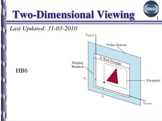
Three-Dimensional Viewing. Jehee Lee Seoul National University. Viewing Pipeline. Virtual Camera Model. Viewing Transformation The camera position and orientation is determined Projection Transformation The selected view of a 3D scene is projected onto a view plane.

E N D
Three-Dimensional Viewing Jehee Lee Seoul National University
Virtual Camera Model • Viewing Transformation • The camera position and orientation is determined • Projection Transformation • The selected view of a 3D scene is projected onto a view plane
General 3D Viewing Pipeline • Modeling coordinates (MC) • World coordinates (WC) • Viewing coordinates (VC) • Projection coordinates (PC) • Normalized coordinates (NC) • Device coordinates (DC)
Viewing-Coordinate Parameters • View point (eye point or viewing position) • View-plane normal vector N
Viewing-Coordinate Parameters • Look-at point Pref • View-up vector V • N and V are specified in the world coordinates
Viewing-Coordinate Reference Frame • The camera orientation is determined by the uvn reference frame u v n
World-to-Viewing Transformation • Transformation from world to viewing coordinates • Translate the viewing-coordinate origin to the world-coordinate origin • Apply rotations to align the u, v, n axes with the world xw, yw, zw axes, respectively u v n
Perspective Projection • Pin-hold camera model • Put the optical center (Center Of Projection) at the origin • Put the image plane (Projection Plane) in front of the COP • The camera looks down the negative z axis • we need this if we want right-handed-coordinates
We get the projection by throwing out the last coordinate: Perspective Projection • Projection equations • Compute intersection with PP of ray from (x,y,z) to COP • Derived using similar triangles (on board)
Homogeneous coordinates • Is this a linear transformation?
Homogeneous coordinates • Trick: add one more coordinate: • Converting from homogeneous coordinates homogeneous viewing coordinates homogeneous projection coordinates
divide by third coordinate divide by fourth coordinate Perspective Projection • Projection is a matrix multiply using homogeneous coordinates: • This is known as perspective projection • The matrix is the projection matrix • Can also formulate as a 4x4
Perspective Projection • The projection matrix can be much involved, if the COP is different from the origin of the uvn coordinates • See the textbook for the detailed matrix
Traditional Classification of Projections • Three principle axes of the object is assumed • The front, top, and side face of the scene is apparent
Perspective-Projection View Volume • Viewing frustum • Why do we need near and far clipping plane ?
Normalizing Transformation • Transform an arbitrary perspective-projection view volume into the canonical view volume • Step 1: from frustum to parallelepiped
Normalizing Transformation • Transform an arbitrary perspective-projection view volume into the canonical view volume • Step 2: from parallelepiped to normalized
Parallel Projection • Special case of perspective projection • Distance from the COP to the PP is infinite • Also called “parallel projection” • What’s the projection matrix? Image World Slide by Steve Seitz
Taxonomy of Geometric Projections geometric projections parallel perspective orthographic axonometric oblique trimetric cavalier cabinet dimetric isometric single-point two-point three-point
Orthographic Transformation • Preserves relative dimension • The center of projection at infinity • The direction of projection is parallel to a principle axis • Architectural and engineering drawings
Axonometric Transformation • Orthogonal projection that displays more than one face of an object • Projection plane is not normal to a principal axis, but DOP is perpendicular to the projection plane • Isometric, dimetric, trimetric
Oblique Parallel Projections • Projection plane is not normal to a principal axis, but DOP is perpendicular to the projection plane • Only faces of the object parallel to the projection plane are shown true size and shape
Oblique Parallel Projections www.maptopia.com
Oblique Parallel Projections • Typically, f is either 30˚ or 45˚ • L1 is the length of the projected side edge • Cavalier projections • L1 is the same as the original length • Cabinet projections • L1 is the half of the original length
Oblique Parallel Projections • Cavalier projections • Cabinet projections
OpenGL 3D Viewing Functions • Viewing-transformation function • glMatrixMode(GL_MODELVIEW); • gluLookAt(x0,y0,z0,xref,yref,zref,vx,vy,vz); • Default: gluLookAt(0,0,0, 0,0,-1, 0,1,0); • OpenGL orthogonal-projection function • glMatrixMode(GL_PROJECTION); • gluOrtho(xwmin,xwmax, ywmin,ywmax, dnear,dfar); • Default: gluOrtho(-1,1, -1,1, -1,1); • Note that • dnear and dfar must be assigned positive values • znear=-dnear and zfar=-dfar • The near clipping plane is the view plane
OpenGL 3D Viewing Functions • OpenGL perspective-projection function • The projection reference point is the viewing-coordinate origin • The near clipping plane is the view plane • Symmetric: gluPerspective(theta,aspect,dnear,dfar) • General: glFrustum(xwmin,xwmax,ywmin,ywmax,dnear,dfar)
Line Clipping • Basic calculations: • Is an endpoint inside or outside the clipping window? • Find the point of intersection, if any, between a line segment and an edge of the clipping window. • Both endpoints inside: trivial accept • One inside: find intersection and clip • Both outside: either clip or reject
1001 1000 1010 Clipping window 0001 0010 0000 0101 0100 0110 Cohen-Sutherland Line Clipping • One of the earliest algorithms for fast line clipping • Identify trivial accepts and rejects by bit operations < Region code for each endpoint > above below right left Bit 4 3 2 1
1001 1000 1010 Clipping window 0001 0010 0000 0101 0100 0110 Cohen-Sutherland Line Clipping • Compute region codes for two endpoints • If (both codes = 0000 ) trivially accepted • If (bitwise AND of both codes 0000) trivially rejected • Otherwise, divide line into two segments • test intersection edges in a fixed order. (e.g., top-to-bottom, right-to-left)
3D Clipping Algorithms • Three-dimensional region coding
Cyrus-Beck Line Clipping • Use a parametric line equation • Reduce the number of calculating intersections by exploiting the parametric form • Notations • Ei : edge of the clipping window • Ni : outward normal of Ei • An arbitrary point PEi on edge Ei
Cyrus-Beck Line Clipping • Solve for the value of t at the intersection of P0P1 with the edge • Ni ·[P(t) - PEi] = 0 and P(t) = P0 + t(P1 - P0) • letting D = (P1 - P0), • Where • Ni 0 • D 0 (that is, P0 P1) • Ni · D 0 (if not, no intersection)
Cyrus-Beck Line Clipping • Given a line segment P0P1, find intersection points against four edges • Discard an intersection point if t [0,1] • Label each intersection point either PE (potentially entering) or PL (potentially leaving) • Choose the smallest (PE, PL) pair that defines the clipped line
3D Clipping Algorithms • Parametric line clipping
Polygon Fill-Area Clipping • Polyline vs polygon fill-area • Early rejection is useful Clipping Window Bounding box of polygon fill area
Sutherland-Hodgman Polygon Clipping • Clip against 4 infinite clip edges in succession
Sutherland-Hodgman Polygon Clipping • Accept a series of vertices (polygon) and outputs another series of vertices • Four possible outputs
Sutherland-Hodgman Polygon Clipping • The algorithm correctly clips convex polygons, but may display extraneous lines for concave polygons
Weiler-Atherton Polygon Clipping • For an outside-to-inside pair of vertices, follow the polygon boundary • For an inside-to-outside pair of vertices, follow the window boundary in a clockwise direction
Weiler-Atherton Polygon Clipping • Polygon clipping using nonrectangular polygon clip windows
3D Clipping Algorithms • Three-dimensional polygon clipping • Bounding box or sphere test for early rejection • Sutherland-Hodgman and Weiler-Atherton algorithms can be generalized
Programming Assignment #2 (3D Viewer) • You are required to implement a 3D OpenGL scene viewer • The viewer should use a virtual trackball to rotate the view • The point of rotation is by default the center of the world coordinate system, but can be placed anywhere in the scene • The viewer should allow you to translate in the screen plane as well as dolly in and out (forward/backward movement) • Your are required to submit a report of at most 3 pages • Describe how to use your program • Describe what you implemented, and what you haven’t
Programming Assignment #2 (3D Viewer) • Virtual trackball • A trackball translates 2D mouse movements into 3D rotations • This is done by projecting the position of the mouse on to an imaginary sphere behind the viewport • As the mouse is moved the camera (or scene) is rotated to keep the same point on the sphere underneath the mouse pointer
Programming Assignment #2 (3D Viewer) • Virtual trackball