Download
1 / 30
310 likes | 616 Views
Model Evaluation. Metrics for Performance Evaluation How to evaluate the performance of a model? Methods for Performance Evaluation How to obtain reliable estimates? Methods for Model Comparison How to compare the relative performance among competing models?. Model Evaluation.

E N D
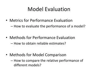
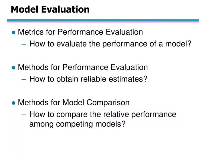
Model Evaluation • Metrics for Performance Evaluation • How to evaluate the performance of a model? • Methods for Performance Evaluation • How to obtain reliable estimates? • Methods for Model Comparison • How to compare the relative performance among competing models?
Model Evaluation • Metrics for Performance Evaluation • How to evaluate the performance of a model? • Methods for Performance Evaluation • How to obtain reliable estimates? • Methods for Model Comparison • How to compare the relative performance among competing models?
Metrics for Performance Evaluation • Focus on the predictive capability of a model • Rather than how fast it takes to classify or build models, scalability, etc. • Confusion Matrix: a: TP (true positive) b: FN (false negative) c: FP (false positive) d: TN (true negative)
Metrics for Performance Evaluation… • Most widely-used metric:
Limitation of Accuracy • Consider a 2-class problem • Number of Class 0 examples = 9990 • Number of Class 1 examples = 10 • If model predicts everything to be class 0, accuracy is 9990/10000 = 99.9 % • Accuracy is misleading because model does not detect any class 1 example
Cost Matrix C(i|j): Cost of misclassifying class j example as class i
Computing Cost of Classification Accuracy = 80% Cost = 3910 Accuracy = 90% Cost = 4255
Accuracy is proportional to cost if1. C(Yes|No)=C(No|Yes) = q 2. C(Yes|Yes)=C(No|No) = p N = a + b + c + d Accuracy = (a + d)/N Cost = p (a + d) + q (b + c) = p (a + d) + q (N – a – d) = q N – (q – p)(a + d) = N [q – (q-p) Accuracy] Cost vs Accuracy
Cost-Sensitive Measures • Precision is biased towards C(Yes|Yes) & C(Yes|No) • Recall is biased towards C(Yes|Yes) & C(No|Yes) • F-measure is biased towards all except C(No|No)
Model Evaluation • Metrics for Performance Evaluation • How to evaluate the performance of a model? • Methods for Performance Evaluation • How to obtain reliable estimates? • Methods for Model Comparison • How to compare the relative performance among competing models?
Methods for Performance Evaluation • How to obtain a reliable estimate of performance? • Performance of a model may depend on other factors besides the learning algorithm: • Class distribution • Cost of misclassification • Size of training and test sets
Learning Curve • Learning curve shows how accuracy changes with varying sample size • Requires a sampling schedule for creating learning curve: • Arithmetic sampling(Langley, et al) • Geometric sampling(Provost et al) Effect of small sample size: • Bias in the estimate • Variance of estimate
Methods of Estimation • Holdout • Reserve 2/3 for training and 1/3 for testing • Random subsampling • Repeated holdout • Cross validation • Partition data into k disjoint subsets • k-fold: train on k-1 partitions, test on the remaining one • Leave-one-out: k=n • Stratified sampling • oversampling vs undersampling • Bootstrap • Sampling with replacement
Model Evaluation • Metrics for Performance Evaluation • How to evaluate the performance of a model? • Methods for Performance Evaluation • How to obtain reliable estimates? • Methods for Model Comparison • How to compare the relative performance among competing models?
ROC (Receiver Operating Characteristic) • Developed in 1950s for signal detection theory to analyze noisy signals • Characterize the trade-off between positive hits and false alarms • ROC curve plots TP (on the y-axis) against FP (on the x-axis) • Performance of each classifier represented as a point on the ROC curve • changing the threshold of algorithm, sample distribution or cost matrix changes the location of the point
At threshold t: TP=0.5, FN=0.5, FP=0.12, FN=0.88 ROC Curve - 1-dimensional data set containing 2 classes (positive and negative) - any points located at x > t is classified as positive
ROC Curve (TP,FP): • (0,0): declare everything to be negative class • (1,1): declare everything to be positive class • (1,0): ideal • Diagonal line: • Random guessing • Below diagonal line: • prediction is opposite of the true class
Using ROC for Model Comparison • No model consistently outperform the other • M1 is better for small FPR • M2 is better for large FPR • Area Under the ROC curve • Ideal: • Area = 1 • Random guess: • Area = 0.5
How to Construct an ROC curve? • Use classifier that produces posterior probability for each test instance P(+|A) • Sort the instances according to P(+|A) in decreasing order • Apply threshold at each unique value of P(+|A) • Count the number of TP, FP, TN, FN at each threshold • TP rate, TPR = TP/(TP+FN) • FP rate, FPR = FP/(FP + TN)
How to construct an ROC curve? Threshold >= ROC Curve:
A Perfect Classifier (0,1) (1/2,1) (1,1) (0,1/2)
Test of Significance • Given two models: • Model M1: accuracy = 85%, tested on 30 instances • Model M2: accuracy = 75%, tested on 5000 instances • Can we say M1 is better than M2? • How much confidence can we place on accuracy of M1 and M2? • Can the difference in performance measure be explained as a result of random fluctuations in the test set?
Confidence Interval for Accuracy • Prediction can be regarded as a Bernoulli trial • A Bernoulli trial has 2 possible outcomes • Possible outcomes for prediction: correct or wrong • Collection of Bernoulli trials has a Binomial distribution: • x Bin(N, p) x: number of correct predictions • e.g: Toss a fair coin 50 times, how many heads would turn up?Expected number of heads = Np = 50 0.5 = 25 • Given x (# of correct predictions) or equivalently, acc=x/N, and N (# of test instances), Can we predict p (true accuracy of model)?
Confidence Interval for Accuracy Area = 1 - • For large test sets (N > 30), • acc has a normal distribution with mean p and variance p(1-p)/N • Confidence Interval for p: Z/2 Z1- /2
Confidence Interval for Accuracy • Consider a model that produces an accuracy of 80% when evaluated on 100 test instances: • N=100, acc = 0.8 • Let 1- = 0.95 (95% confidence) • From probability table, Z/2=1.96
Comparing Performance of 2 Models • Given two models, say M1 and M2, which is better? • M1 is tested on D1 (size=n1), found error rate = e1 • M2 is tested on D2 (size=n2), found error rate = e2 • Assume D1 and D2 are independent • If n1 and n2 are sufficiently large, then • Approximate:
Comparing Performance of 2 Models • To test if performance difference is statistically significant: d = e1 – e2 • d ~ N(dt,t) where dt is the true difference • Since D1 and D2 are independent, their variance adds up: • At (1-) confidence level,
An Illustrative Example • Given: M1: n1 = 30, e1 = 0.15 M2: n2 = 5000, e2 = 0.25 • d = |e2 – e1| = 0.1 (2-sided test) • At 95% confidence level, Z/2=1.96=> Interval contains 0 => difference may not be statistically significant
Comparing Performance of 2 Algorithms • Each learning algorithm may produce k models: • L1 may produce M11 , M12, …, M1k • L2 may produce M21 , M22, …, M2k • If models are generated on the same test sets D1,D2, …, Dk (e.g., via cross-validation) • For each set: compute dj = e1j – e2j • dj has mean dt and variance t • Estimate: