Download
1 / 24
270 likes | 505 Views
Consumption. Important for the study of both growth and cycles Has been at the center of many important empirical analysis Plan: Romer (2012) Chapter 8. Why studying consumption?. Consumption under Certainty: Life-Cycle/Permanent-Income Hypothesis.

E N D
Consumption • Important for the study of both growth and cycles • Has been at the center of many important empirical analysis • Plan: Romer (2012) Chapter 8 Why studying consumption?
Consumption under Certainty: Life-Cycle/Permanent-Income Hypothesis Modigliani-Brumberg (1954) and Friedman (1957) Developed in reaction to the empirical problems coming out of Keynes (1936) consumption function • Presented in Romer with many simplifying assumptions • Individual living for T period • Initial wealth of A0 • Interest rate and discount rate set to zero (see fn 1, page 366) • Labour income of Lifetime utility function: Individual can save and borrow
Individual budget constraint: The Lagrangian is: First-order condition for Ctis: This hold for any period (r-ρ=0) so Ct is constant and from 8.2:
Consumption is a function of permanent incomeYP the right-hand side of 7.5. Transitory income is the difference between current income Yt and permanent income. One time income of Z raises consumption by Z/T Temporary income tax cut has a small effect on consumption. The time pattern of income is not important for consumption But it is fundamental for Saving S:
Empirical applications: Understanding Estimated Consumption Function The traditional Keynesian consumption function is: Where Y is current income. The stable and consistent relationship was rejected in some important empirical studies. Three cases to consider Ci 1) The Keynesian C function was not rejected in pure cross-sectional studies (across household, at one point in time) 45o Yi
Ct But rejected in time-series of one country over a long period of time 45o Yt Ci And the cross-section consumption function differs across groups Whites Blacks 45o Yi
In a celebrated paper, Friedman (1957) demonstrate that the permanent income hypothesis provides and explanation for the three sets of facts. Suppose that the true model is C = YPand current income Y=YP + YT Suppose that YThas a mean zero and is uncorrelated with permanent income Consider a regression based on the wrong model: Where, in OLS: Given that:
Furthermore, the estimated constant equals: • For cross-section studies, Var(YT) (coming from u and differences • in their life-cycle) is comparable with Var(YP), consequently, • b is smaller than 1 and ais positive.
2) In time series, most of the Var(Y) is associated with long-run growth and b is close to one and a close to zero. 3) As for the differences between blacks and whites, their relative Var are the same but: Read carefully the discussion on page 371.
Consumption under Uncertainty: Hall’s Random-Walk Hypothesis Introducing uncertainty and suppose the u function is quadratic. Then, the individual maximizes: Under budget constraint 7.2 Here Romer use the same approach than he used for the Euler equation. A consumer on its optimal path: Where E1stands for the expectation based on information available at time 1.
Then, we get: And taking the expectation on both sides of the budget constraint and using 8.12, we get: Since by definition of expectations: Where the expectation of et is zero, 8.15 and 8.12 imply:
Hall’s (in)famous result (see fn6 page 375) Permanent income hypothesis imply that only unexpected event can affect consumption. Expected event are smoothed by for-sighted agents. Empirical applications: testing the random-walk hypothesis • Hall’s approach: regress the changes in C (t-1,t) on variables • that are known at time t. For example lag changes in income. • This could be easily done in EViews with Granger causality test
Pairwise Granger Causality Tests Date: 11/06/03 Time: 16:25 Sample: 1953:1 1984:4 Lags: 4 Null Hypothesis: Obs F-Statistic Probability DLY does not Granger Cause DLCS 123 1.04969 0.38489 DLCS does not Granger Cause DLY 6.77287 6.3E-05 Simple test using consumption and income data in Green, 4th edition databank (CD) from US data. The null is not rejected in the first row. Consequently, the null of Random Walk is not rejevted. Similarly, with 5 lags:
Pairwise Granger Causality Tests Date: 11/06/03 Time: 16:28 Sample: 1953:1 1984:4 Lags: 5 Null Hypothesis: Obs F-Statistic Probability DLY does not Granger Cause DLCS 122 1.18578 0.32076 DLCS does not Granger Cause DLY 5.57381 0.00013 But this approach was criticized by Campbell and Mankiw (1989b). AS Romer (2001) puts it: “Hall’s result that lagged income does not have strong predictive power for consumption could arise not because predictable changes in income do not produce predictable changes in consumption but because lagged values of income are of little use in predicting income movements.”
Campbell and Mankiw suppose that the fraction λ of households consume their current income and the other follow Hall’s consumption. Consequently, they want to test: Where et is the change in households’ estimate of their permanent income between t-1 and t. But Ztand et are correlated!! (explanation) Then the right-hand side independent variable is correlated with the error term. In this case, OLS estimates might be biased (and the variance not accurately estimates). In such a case, the approach is to use instrumental variables (IV). Instruments are variable correlated with the right hand side variable but not correlated with the residual.
This is simply done with two-stage least squares (as done in the book). The first regression is a regression of Zt on the instruments. The second regression is a regression of the left-hand side variable on the fitted values of Z: Often, as in this case, the instruments are lagged variables. Campbell and Mankiw find that lagged changes in income has no predictive power for future changes (putting doubts on Hall’s empirical analysis). As a base case, they use lagged changes in consumption as instruments. Romer reports estimates of λ of 0.42 (0.16) and 0.52 (0.13) for three and five lags respectively.
Dependent Variable: DLCS Method: Two-Stage Least Squares Date: 11/04/03 Time: 17:02 Sample(adjusted): 1954:1 1984:4 Included observations: 124 after adjusting endpoints Instrument list: C DLCS(-1) DLCS(-2) DLCS(-3) Variable Coefficient Std. Error t-Statistic Prob. C 0.006187 0.001710 3.618526 0.0004 DLY 0.294314 0.178857 1.645522 0.1024
Dependent Variable: DLCS Method: Two-Stage Least Squares Date: 11/04/03 Time: 17:02 Sample(adjusted): 1954:3 1984:4 Included observations: 122 after adjusting endpoints Instrument list: C DLCS(-1) DLCS(-2) DLCS(-3) DLCS(-4) DLCS(-5) Variable Coefficient Std. Error t-Statistic Prob. C 0.004460 0.001671 2.668920 0.0087 DLY 0.487123 0.166591 2.924062 0.0041 Read carefully the remaining of 7.3
The interest rate and consumption. What happen if interest rate and discount rate non null We already know, follow Romer analysis in 8.4. (redo it yourself) when he get the now well known Euler equation (in discreet time): They could be a trend in the consumption depending on r - ρ
But the effect of an increase in the interest rate is not necessarily to decrease saving since there is two effect; a substitution effect (which tend to increase saving) Analyse by your-self the discussion related with Figure 7.2 on page 347. You have to be able to redo it at the exam.
The interest rate and saving • Although an increase in the interest rate at period t reduce the ratio of consumption at period t + 1 over consumption at period t , it does not mean that saving is increased at period 1. • Change in the interest rate have a substitution and an income effect. • Best illustrated graphically with a 2 period model. • Assume the individual has no initial wealth. • The individual budget constraint go through the point Y1 – Y2. • The slope of the budget constraint is –(1+r).
2 – Saving is initially positive: both a substitution and an income effect – effect on saving ambiguous
3 – Borrowing initially: both substitution and income effect work in the same direction – saving rise