Download
1 / 11
240 likes | 781 Views
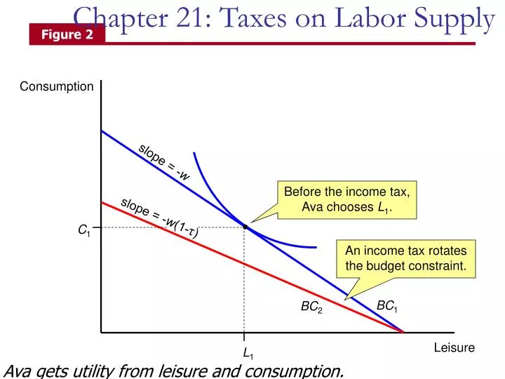
Chapter 21: Taxes on Labor Supply. Figure 2. Consumption. slope = - w. Before the income tax, Ava chooses L 1. slope = - w (1- τ ). C 1. An income tax rotates the budget constraint. BC 1. BC 2. Leisure. L 1. Ava gets utility from leisure and consumption.

E N D
Chapter 21: Taxes on Labor Supply Figure 2 Consumption slope = -w Before the income tax, Ava chooses L1. slope = -w(1-τ) C1 An income tax rotates the budget constraint. BC1 BC2 Leisure L1 Ava gets utility from leisure and consumption.
Taxes on labor supply – TheoryBasic Theory • Ava’s initial budget constraint, the blue line, is initially expressed as: • Where the price of consumption goods is normalized to unity, and T is the full time endowment. • She initially chooses bundle A, that is (L1,C1).
Taxes on labor supply – TheoryBasic Theory • After a proportional income tax is introduced, her budget constraint rotates downward to the red line, becoming: • For any given amount of work effort, Ava would be able to purchase fewer consumption goods. • Ava’s wage rate falls from w to (1-J)w.
Labor Supply: suppose wages fall to $7.50 from $15 an hour 1200 In this example, wages fall and you work more. The IE is larger than the SE and the labor supply curve is backward bending. Income $ 600 SE IE 80 38 45 60 Leisure Hours of work
Labor Supply: suppose wages fall to $7.50 from $15 an hour 1200 In this example, wages fall and you work less. The IE is smaller than the SE and the labor supply curve is upward sloping. Income $ 600 SE IE 45 80 60 52 Leisure Hours of work
The SE is larger than the IE: The IE is larger than the SE: Labor Supply and Income and Substitution Effects Wages Wages Individual labor supply curve Individual labor supply curve 20 60 40 10 40 35 20 40 Q of labor (hours) Q of labor (hours)
Figure 3 Make sure you can identify income and substitution effects! Consumption Consumption Income effect of a tax increase is larger Substitution effect of a tax increase is larger Ava works less. Ava works more. C1 C1 C2 C2 BC1 BC2 BC1 BC2 Leisure Leisure L2 L1 L2 L1
Taxes on labor supply – TheoryBasic Theory • In the first picture, Ava consumes more leisure and less hours of work. Here leisure increases from L1 to L2. In this case, the substitution effect is larger than the income effect. • In the second picture, Ava consumes less leisure and more hours of work. Here leisure decreases from L1 to L3. In this case, the substitution effect is smaller than the income effect. • At low levels of labor supply, it seems very unlikely that income effects could be larger than substitution effects, because the income effects are proportional to hours worked before the wage change.
Taxes on labor supply – TheoryLimitations on the theory • The basic labor supply theory is an “idealized view” of the labor market. In reality, a number of additional constraints factor in. • For example, it is unlikely that individuals can freely adjust their hours of work. • In addition, constraints like overtime pay change the budget constraint. • Overtime pay rules mean that workers in most jobs must legally be paid one and a half times their regular hourly pay if they work more than 40 hours per week. • These rules create a non-convexity in the budget constraint, and make it expensive for firms to hire workers for more than 40 hours per week. • At the same time, most people choose what jobs and therefore what hours to work.
Taxes on labor supply – Evidence • The empirical literature on taxation and labor supply makes a distinction between two kinds of workers. • Primary earners are the family members who are the main source of labor income for a household. • Secondary earners are workers in the family other than the primary earners. • Traditionally, primary earners are thought of as husbands and secondary earners as wives who were in charge of child care.
Taxes on labor supply – Evidence • The general conclusions from econometric studies are that: • Labor supply elasticities for primary earners are around +0.1, a fairly small effect. • Labor supply elasticities for secondary earners are in the range of +0.5 to +1.0, a much larger effect. This effect comes mainly from the extensive margin of whether to work or not, rather than the intensive margin on the actual number of hours to work.