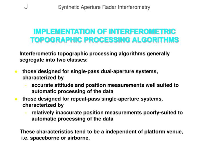
IMPLEMENTATION OF INTERFEROMETRIC TOPOGRAPHIC PROCESSING ALGORITHMS

1. IMPLEMENTATION OF INTERFEROMETRIC TOPOGRAPHIC PROCESSING ALGORITHMS Interferometric topographic processing algorithms generally segregate into two classes: • those designed for single-pass dual-aperture systems, characterized by • accurate attitude and position measurements well suited to automatic processing of the data • those designed for repeat-pass single-aperture systems, characterized by • relatively inaccurate position measurements poorly-suited to automatic processing of the data These characteristics tend to be a independent of platform venue, i.e. spaceborne or airborne.

2. PROCESSOR ARCHITECTURES • Single-pass two aperture implementations tend to segregate further into several classes of processors • Fully automated strip mode processors that carry raw data to an arbitrarily long height strip (e.g. ARPA TOPSAR) • relatively inflexible • usually tailored to problem at hand • optimized for speed and efficiency (minimal disk; much RAM) • Fully automated but scene-oriented processors that produce height maps on a scene by scene basis (NASA AIRSAR; CCRS?) • more flexible; less efficient • Modular scene oriented processors that work well for single pass or repeat pass • very flexible; least efficient

3. INTERFEROMETRIC PROCESSING FLOW DIAGRAM

4. PROCESSOR IMPLEMENTATIONS • Modern SAR interferometry implementations are typically • software processors, with the possible exception of front-end data decoding hardware • coded in high level languages such as C or Fortran • parallelized for multiprocessor environments • workstation compatible • protected by institutional patents and profit motives • Real-time on-board implementations will be feasible in the near future • with military, commercial, and planetary applications • sustained processor speed required: roughly 1-4 GFlOp/sec • commercial multiprocessors are approaching these rates

5. PROCESSING REQUIREMENTS

6. MOTION PROCESSING • Motion measurement systems of the NASA DC-8 are commercially available (though expensive) and support automated processing • Six-Gun GPS receiver used to time tag pulse data to 1/2 PRI • HoneywellH764P-code combined GPS/INU • 1 cm/s velocity • 3 m position long term • 0.001°- 0.005° attitude • motion data time tagged with GPS time • Turbo-Rogue differential GPS data (10 cm accuracy at 1 Hz) • Motion processing entails straightforward transformation of the position and velocity measured in WGS-84 and attitude angles measured in local geoid coordinates (TCN) to the (s,c,h) coordinate system. • Transformations provided in Coordinate Systems module

7. ATTITUDE MOTION PROCESSING • Attitude angles define a transformation taking the fixed interferometric baseline in the platform body-fixed frame, or more precisely the lever arms from the inertial reference to the antenna phase centers, into their orientation with respect to the local (s,c,h) system. Where D is a diagonal matrix with +1 or =1 on diagonals, and Y, P and R are Yaw, Pitch, and Roll rotation matrices, respectively • Details of the sign conventions for the rotation angles and axis scaling depends on the specific choice of reference frames • Transformation matrix M is a function of along track position, and is conveniently pre-tabulated against position for use by the interferometric processor

8. RANGE COMPRESSION AND PRESUMMING • Radar systems typically operate with • constant Pulse Repetition Frequency (PRF) (variable ground sample spacing depending on platform velocity variations) • constant ground sample spacing (variable PRF depending on velocity variations) • To regularize the image coordinates to match the (s,c,h) system, or to simply resample data to some desired reference spacing, variable rate presumming can be invoked • Presumming of pulses most conveniently performed after range compression of pulses. After compression, • data are represented as single-sided spectrum (analytic signal representation), allowing convenient band-pass filtering • scatterer energy is localized in range

9. PRESUMMING FORMULATION

10. MOTION COMPENSATION • Motion compensation of radar data is required for accurate airborne interferometers • Uncompensated motion errors lead to image defocusing and mis-registration, reducing interferometric correlation and height acuity • Motion compensation consists of adjusting the range and phase of each image sample to seem as though the imaging positions lie on the reference track(s)

11. ERRORS RELATED TO MOTION COMPENSATION • If motion compensation is not performed, • Image focusing errors • Common FFT-based focusing algorithms assume platform moves rectilinearly • Without motion compensation, the chirped matched filter assumed in azimuth processing is not matched. • Focussing error reduces the effective number of looks available for processing, and adds sidelobe energy to unweighted processing schemes • No interferometric biases or variance increase if channel processing is identical! • If motion compensation is performed, there are three categories of compensation-induced errors: • Image processing induced phase errors • Unknown terrain errors • Intrinsic measurement errors

12. MOTION COMPENSATION APPROACHES • Dual reference track approach - range and phase corrections applied to each channel to independent references

13. MOTION COMPENSATION APPROACHES • Single reference track approach - range and phase corrections applied to each channel to common reference

14. MOTION COMPENSATION AND INTERFEROGRAM FLATTENING • The equations describing motion compensation and baselines for interferometry are identical. • The range-dependent phase shift introduced in motion compenstion is nothing more than than an interferometric phase due to a curved earth for a fictitious baseline from the reference track to one antenna • In the single reference track approach, the difference of the range-dependent phase shifts between the two channels is then the true “curved-earth” interferometric phase. Thus, motion compensation to a single track automatically removes the “curved-earth” fringes • This process (nearly linear phase ramp in range) shifts the spectra of the two channels in opposite directions, essentially aligning the common parts of their spectra • Suitable low-pass filtering of the common spectral band will enact the spectral shift filtering for the curved-earth

15. MOTION COMPENSATION STRATEGY • Patch-oriented motion compensation allows update of reference track(s) to ensure the actual track is nearby • usual method: pick a patch-local track intersecting at least one point on the actual track and parallel to a global track • reduces unknown terrain errors • usually required for airborne systems subject to variable winds • only cost is in local patch-oriented book-keeping • Global motion compensation defines reference track(s) for entire processing run • usually preferred for spaceborne systems, where motion is smooth • often spaceborne “motion compensation” is simply SLC image co-registration

16. RANGE MIGRATION AND AZIMUTH COMPRESSION • No interferometric issues are peculiar to azimuth processing • In azimuth processing, a choice must be made as to whether or not the pointing will be corrected for squinted imaging • Deskewing generally adds complication to the buffering scheme employed in the processor, but renders the processed imagery in the desired output along track coordinate frame (if the centroid is known precisely) • Skewed processing leaves imagery in natural range-doppler coordinates and allows straightforward height reconstruction (see Height Reconstruction module) • ARPA processor employs squinted processing

17. INTERFEROGRAM FORMATION AND CORRELATION • In implementations with proper automated motion compensation, interferogram and correlation formation consists of simple point-by -point cross multiplication and look summation • In this example, look summation was performed only in the along track direction. Typically, azimuth SLC resolution is finer than range resolution, so looks taken in azimuth “square” the pixels.

18. INTERPOLATION FILTERS • Interpolation filters are employed in • presumming • motion compensation • range migration correction • absolute phase determination • Interpolation filters for all of these critical operations must have the following characteristics • bandwidth preserving, especially the three range dependent interpolators • low order polynomials won’t do! • phase and time delay preserving, especially in motion compensation where misalignment amounts to decorrelation • nearest neighbor won’t do! • Interpolator filter design a rich subject

19. PHASE UNWRAPPING • Elements of the phase unwrapping problem: From the measured, wrapped phase, unwrap the phase from some arbitrary starting location, then determine the proper ambiguity cycle. Actual phase Wrapped (measured) phase Typical unwrapped phase

20. TWO-DIMENSIONAL PHASE UNWRAPPING • Two dimensional phase field values below are in units of cycles • One-dimensional unwrapping criterion of half-cycle proximity is inconsistent in two dimensions • Residues, marked with + and -, define ambiguous boundaries.

21. RESIDUES IN PHASE UNWRAPPING • The wrapping operator delivers the true phase modulo 2 , in the interval - <  < . • The true phase gradient is conservative: • The wrapped gradient of the measured, wrapped phase, however, may not be conservative: • When this function is non-conservative, its integration becomes path dependent. • Residues occur at locations of high phase noise and/or phase shear such that the wrapped gradient of the measured, wrapped phase is no longer conservative.

22. BRANCH CUTS IN PHASE UNWRAPPING • Branch-cut algorithms (Goldstein, Zebker, and Werner 1986) seek to neutralize these regions of inconsistency by connecting residues of opposite solenoidal sense with cuts, across which integration may not take place. • Branch cut connections force path independence in the integration of the wrapped phase gradient. • If done properly, the integrated phase field will be correct. But which is correct?

23. ILLUSTRATION OF BRANCH CUT ALGORITHM • Connection of simple tree

24. BRANCH CUT STRATEGY • The standard GZW algorithm is designed to connect residues into a neutral network into the shortest possible connection tree, i.e. to minimize the length of the individual branch cuts comprising a tree • This will not necessarily create the shortest possible tree, since GZW makes many unnecessary connections in its search for neutrality • Various criteria have been devised to place guiding centers (unsigned residues) along expected paths to facilitate the right choice in branch cut connection Residues Guiding Centers

25. GUIDING CENTER CRITERIA • A number of criteria have been devised for selecting guiding centers, each more or less tailored to characteristics of SAR data: • when phase slope exceeds threshold (implies layover) • when derivative of phase slope exceeds threshold • when radar brightness exceeds threshold (implies layover) • when decorrelation estimator exceeds threshold (implies noise and/or layover • Some guiding center selections help in some cases • Difficult to assess performance in a qauntitative way

26. LEAST SQUARES PHASE UNWRAPPING • In recent years, linear least squares algorithms (Ghighlia et al, 1994) have become popular • Numerous challenges to primacy of branch cut algorithms have been made, because branch cut algorithms are not robust in noise and performance is difficult to assess. • Premise of least squares algorithm: • Model the non-conservative component of as noise term in a least squares problem: Problem can expressed in terms of Poisson’s equation which lends itself to fast numerical solution (when unweighted)

27. LEAST SQUARES PHASE UNWRAPPING • Numerous researchers have been finding significant biasing of the phase estimates from the least squares method. • Slopes tend to be underestimated • Large-scale warping of the phase field • Cause of distortion (attributed to Bamler et al, 1996 preprint) • Least square condition of zero-mean uncorrelated gaussian noise is violated. • Error function is signal dependent, and a nonlinear function of the original noise corrupting the signal. Mean of error function is related to the signal, biasing result. • Recent work by Zebker et al is showing that least squares works well when combined with branch cuts, as it must. • Other algorithms exist but are generally variants on branch cuts or least squares

28. PHASE UNWRAPPING IMPLEMENTATION • In patch oriented processing schemes, it is convenient to “bootstrap” the unwrapped phase from one patch to the next • Occasionally, when unwrapping is difficult, “bootstrapping” can be essential to success

29. ABSOLUTE PHASE DETERMINATION • There are at least three methods for determining the absolute phase ambiguity Actual phase Wrapped (measured) phase Typical unwrapped phase

30. ABSOLUTE PHASE DETERMINATION METHODS • Ground control reference points can be used to determine the absolute phase ambiguity

31. ABSOLUTE PHASE DETERMINATION METHODS • The spectral method of absolute phase determination (Madsen et al., 1992) divides the imagery into two range sub-bands, forming one lower resolution interferogram in each sub-band • The difference of sub-banded interferograms gives a new interferogram with an effective fringe frequency scaled down from the original full resolution interferogram by • The fringe frequency is so low that unwrapping is not necessary • This phase scaled up by the inverse frequency ratio is very noisy • The difference between this phase and the unwrapped phase, averaged over a large area to reduce noise, gives the ambiguity

32. ABSOLUTE PHASE DETERMINATION METHODS • The range-correlation method of absolute phase detrminion (Madsen, 1995) exploits spatial domain misregistration • Interferometric phase is a record of pixel mis-registration: • Topographic phase also contributes to small variable mis-registration • Unwrapped phase can be used to remove the topographic mis-registration by resampling one image to match the other through above prescription • If unwrapped phase is on the correct ambiguity, then images will align precisely - no mis-registration will be detected in cross-correlation of imagery • If ambiguity is incorrect, cross-correlation will measure a constant offset throughout the image. Average the estimates over the image yields the scaled ambiguity estimate.

33. ABSOLUTE PHASE METHOD ASSESSMENT • The performance of all methods is highly dependent on the system performance characteristics • Both spectral and correlation methods rely on averaging of noisy data • Estimator performance characteristics can be modeled and a system designed to meet the required specification • Ground control point method requires access to DEM or ground control wherever the data are taken • All methods require system stability to a few degrees of phase

34. • • • • • • ••• • • • • • • • • •  • • • • • ••• • • • • • • • • • •• • •  • • • • •• • • • •• • • • • • • • • • • • • • • • • • • • • • • • • • • • • • • • • • • • • • • • • • • • • • • • • Interpolator • • • • • • • • • • • • • • • • • • • • • • • • • • • • • • • • • • • • • • • • • • • • • • • • • • • • • • • • • • • • • • • • • • • • • • • • • • • • • • • • REGRIDDING IN GEOLOCATION Position vectors are not uniformly distributed in the plane following height reconstruction process. Use some interpolator to resample to a uniform grid.

35. REGRIDDING INTERPOLATORS IN GEOLOCATION • Interpolating noisy, irregularly spaced data to a uniform grid is a difficult problem. • Several interpolation algorithms have been implemented • Aikima interpolator - triangulates the surface. Fits a 5th degree polynomial over each triangle, forcing continuity of the first and second partials along all triangle edges. Method is sens-itive to noise and requires a great deal of memory and time. • Nearest neighbor - Fast and easy, but shows some artifacts in shaded relief images. Potential exists for biasing height estimates when data are noisy but regularly laid out on output grid.

36. MORE REGRIDDING INTERPOLATORS • Another implementation: • First or second order surface fitting - Uses the height data centered in a box about a given point and fits a surface by weighted least squares. • Fit weighted by distance from point and height noise (as determined from the interferometric correlation). • Box size determined by local topography: small height variations large box - large variations use small box. • Another benefit to the surface fitting method is slope and/or surface curvature maps are readily available from the fit coefficients directly using the unresampled data. • Efficient implementation achieved by storing the position vectors in an array structured a(3,M,N) where the location in the array is determined using a nearest neighbor algorithm.

37. SURFACE FITTING BENEFITS • Slope and Curvature Images of Galapagos Islands

38. REPEAT-PASS SINGLE-APERTURE INTERFEROMETER IMPLEMENTATIONS • Repeat pass implementations are distinguished by insufficient position accuracy to allow automated processing • For spaceborne platforms, orbits traditionally have been determined to no better than tens to hundreds of meters. In this case, the data themselves must be used to determine the interferometric baseline • Modern spaceborne systems such as ERS, SIR-C are producing reconstructed orbit solutions that approach meter -level accuracy or better. Some automation, through interferogram formation at least, is possible when the orbit accuracy is sub-pixel. • Airborne systems can achieve cm-level track accuracy if equipped with differential kinematic GPS processing. However, geometry usually requires mm level accuracy for accurate topographic mapping.

39. REPEAT-PASS PROCESSOR ARCHITECTURES • Repeat pass interferometric processors are typically “scene-” or “frame-based”, working from data processed to single look complex (SLC) imagery at the agency processing facilities, or from raw data processed locally. Interferometric processing could be done in GIS-based software or with an image processing tool suite, though perhaps not efficiently. • With accurate interferometric baseline knowledge (or equivalently the SLC coregistration offset field), it is possible to process from raw signal samples to as far down the chain as accuracy and data quality permit • Arbitrarily long swaths can be processed efficiently through the interferogram level. • Further processing usually an iterative process

40. FLEXIBLE REPEAT PASS INTERFEROMETRY Procedure to pre-determine offsets: process first and last piece of data, then interpolate offsets between

41. SCENE MATCHING AND COREGISTRATION • Cross-correlate images by expedient method

42. SCENE MATCHING ON IMAGERY • There are a plethora of algorithms in existence for automatic scene matching, each with particular strengths and weaknesses • SAR scenic matching for interferometry applications is difficult for several reasons: • Thermal noise causes the fine structure of two SAR images to differ, adding noise to the correlation measurements. • Geometric speckle noise is similar in images acquired in nearly the same geometry, but as the interferometric baseline increases, differing speckle noise corrupts the matching correlation. • Scene decorrelation is another form of speckle noise difference that corrupts matching correlation. • SAR scenic matching for mosaicking applications involves greater challenges, including severe speckle noise differences, layover and shadow effects.

43. d Search Window AUTOMATIC SCENE MATCHING • Find overlap region and sample points at specified spacing in along track and cross track direction. • Typical window sizes are 64x64 pixels for image data and 64x64 or 128x128 pixels for height data. • Uses a modified Frankot's method for rejecting bad matches and to provide an estimate of the match covariance matrix. • Cross correlation uses a normalized mean correlation function, mean of search window is calculated over the region in common with the reference window. Mean of reference is constant Mean of search varies with position

44. MATCH CORRELATION ESTIMATE • Correlation is computed in the spatial domain using a normalized cross correlation algorithm. • Let be the image values at a point in the reference window in the first data set, , the mean of the intensities in that window. • Let be the image value at point in the search window of the second data set, and the mean of the intensities in that window. • Viewing each image as a vector in an n-dimensional vector space then the cross correlation is computed as where and are the standard deviations of the image intensities in data sets 1 and 2, respectively. Space-domain correlation used for speed and because large irregular data gaps are trouble free.

45. Solve two equations for two unknowns: • Evaluating baseline at several widely-spaced along-track (azimuth) locations gives azimuth history of the baseline. BASELINE ESTIMATION FROM OFFSETS • Baseline estimation in repeat pass interferometry is a rich subject, and will be covered completely in a separate module. Briefly: • Offset field determined from scene matching carries information sufficient to reconstruct the baseline to an accuracy com-mensurate with ability to co-register images. • For nearly parallel, smoothly varying, orbit tracks, the baseline can be modeled as a simple function of the range

46. BASELINE ESTIMATION FROM OFFSETS • For orbit tracks with substantial convergence, azimuth offsets strongly characterize convergence rates. Observation vector: Parameter vector: where  is an image scaling factor resulting from velocity differences between the tracks, and (s,c,h) are local coordinates defined by the orbit track (see notes on coordinate systems).

47. BASELINE ACCURACY FROM OFFSETS • Baselines determined from offset fields are typically accurate to a fraction of the scene matching accuracy that depends on the model function and the number of offset estimates. Example: • Zero baseline image pair with 10 match points across range. • Scene matching accuracy of 1/20 pixel resolution at typical single look resolution of 15 meters: 75 cm / 25 cm • This accuracy is insufficient for topographic mapping applications These geometric parameters are typical of ERS with baselines suitable for topography. Generally, ground control points tied to the unwrapped interferometric phase are required for mapping.

48. INTERFEROGRAM FORMATION Doppler spectra matched during processing From interferogram and detected imagery, corr- lation can be formed properly at any resolution: i.e. average of correlation is not correlation of average

49. REGISTRATION IMPLEMENTATION • In resampling single look complex image to register properly with the reference image, care must be taken in interpolation of complex data • The azimuth spectrum of squinted SAR data is centered at the Doppler centroid frequency - a band-pass signal • Simple interpolators, such as linear or quadratic interpolators, are low-pass filters and can destroy band-pass data characteristics • Band-pass interpolators or spectral methods preserve phase fidelity

50. INTERFEROGRAM RANGE OVERSAMPLING • Several references recommend oversampling single look complex data in range before forming the interferogram, arguing • each SLC is a full bandwidth signal • product of two signals forms a new signal whose spectrum is the convolution of individual spectra, hence has spectral content beyond the Nyquist sampling frequency in range. • In practice, oversampling is unnecessary because • there is no appreciable improvement in performance • each SLC usually utilizes less than 80% of the bandwidth • spectral shift filtering reduces the bandwidth further • noise from aliased energy usually inconsequential relative to decorrelation noise