Download
1 / 21
210 likes | 325 Views
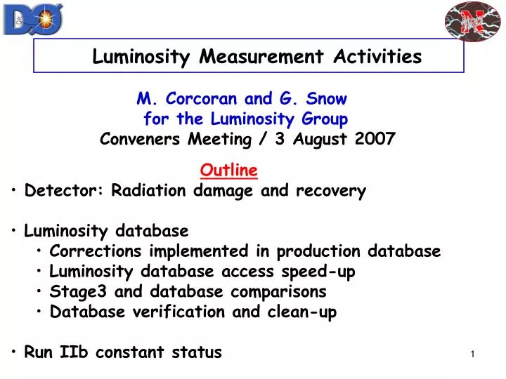
Luminosity Measurement Activities M. Corcoran and G. Snow for the Luminosity Group Conveners Meeting / 3 August 2007. Outline Detector: Radiation damage and recovery Luminosity database Corrections implemented in production database

E N D
Luminosity Measurement Activities M. Corcoran andG. Snow for the Luminosity Group Conveners Meeting / 3 August 2007 • Outline • Detector: Radiation damage and recovery • Luminosity database • Corrections implemented in production database • Luminosity database access speed-up • Stage3 and database comparisons • Database verification and clean-up • Run IIb constant status
constant, if no radiation damage From May 18 conveners talk: Light output of LM scintillators is steadily deteriorating Yugi Enari since beginning of Run IIb
Oxygen Annealing a Success • Annealing effect • From 11th July,13:00, nitrogen purge for LM was replaced with dry air • Clearly see annealing effect of the oxygen, all scintillators similar • The recovery now looks saturated • LM scintillators will be replaced during this shutdown 200.7.26 2007.7.11 Yugi Enari
Forward Muon Special Runs • D periodically takes special runs triggering on single muons • measured in the forward muon detectors for monitoring purposes • A pseudo cross-section called the “muon yield (Y)” is calculated: • Number of reconstructed muons • Y = • Integrated luminosity in special run • An uncertainty of about 1% (stat + syst) is estimated for the • numerator in each muon yield calculation • The muon yields can potentially reveal instabilities in the luminosity • measurement • The following plots show normalized yields defined as • Ynorm = Y / (mean value)
1% Ynorm Normalized muon yield July 11 2006 June 24 2007 • Forward muon yields show stability within 1% during Run IIb
Ynorm Normalized muon yield Instantaneous L • Special runs taken during 2 stores in late 2006 • November 29 (Linitial = 105E30) and December 12 (Linitial = 229E30) • Note absence of instantaneous luminosity dependence
Final corrections implemented in production database (Delivered L only here) Period A Period B Period C Periods E + E’ Period F Period D Correction = 1.00 Plotted: Line = Correction function vs. delivered instantaneous luminosity Points = Corrected luminosity / Uncorrected luminosity vs. uncorrected delivered “Outlying LBNs” (showing greater L than ever delivered for a given period) are understood as stemming from unusable, non-physics runs E. Gallas, K. DeVaughan
Thanks to Elizabeth Gallas A thanks to Elizabeth Gallas was posted in D0News on July 30 for her work implementing the corrections in the database. Hours of tireless volunteer work over the last few months. Real work ended June 15, but she is still plugged in. My machine shop is preparing a gift – desk ornament made from Run IIa LM scintillators mounted on an engraved base. (Don’t tell her!) Igor Mandrichenko has taken over DB offline maintenance and has inherited DB run report code from Ana in Brazil.
New lm_access tools for retrieving database luminosity Stage3 retrieval about a factor of 2 faster than database LBNs/second retrieved • Luiz Mundim’s (+ others) new tools to speed retrieval of luminosity • information from the database by a factor of ~100 are essentially ready • to go. Example: Run IIa data set – 2.5 hours Stage3, 5 hours database for • 1 trigger. • Observation: Database retrieval depends on client machine (5 hours above • using DB server, 3.75 hours on Luiz’s Clued0 box.) • Luiz also testing multiple users hitting DB – not a big issue due to low usage. • Next step for these tools: Run on development instance, then ready for • production instance. (S. White) • Release expected when next two steps are complete (about 1 month).
Database/Stage3 comparison status • V. Malyshev has done a thorough comparison of the recorded • luminosity for the entire Run II data sample, using groups of • runs. • Our general aim: investigate discrepancies greater than 0.5%. • Examples: • Run range: 221694-224486 DB: 58.6526pb-1Stage3: 58.6654pb-1 • DB 0.02% smaller than Stage3 • Run range: 226073-229706 DB: 211.547pb-1Stage3: 211.271pb-1 • DB 0.13% larger than Stage3 • Run range: 229707-230270 DB: 94.6721pb-1 Stage3: 82.9074pb-1 • DB 14.2% larger than Stage3 – tracked down to missing • Stage3 files • Luiz has made a new script to do detailed LBN by LBN comparisons • so we can understand both large and very small differences. • Work to be done by Luiz, Marj, Greg, Kayle since Vladimir will • be consumed by shutdown work. • This will also shed light on the last issue ……………….
Database verification and clean-up • J. Linnemann and S. White are investigating the database • content, entry-by-entry. • The DB contains many more error and status messages/flags • compared to the stage3 LBN-level status flags • Jim: DB has 1.1 billion trigger status messages. • Example: “Such-and-such trigger did not fire during this LBN’s • duration”. • Lm_access only checks LBN-level status messages to decide whether • to include or throw out an LBN in an integrated lumi calculation. • Tasks: • Determine whether any important status messages in DB are missed • by lm_access, whether they are redundant, useless, etc. • Decide fate of additional status flags in DB – delete, clean up, • quit writing them, pay attention to them, etc. • One month time scale.
Run IIb Normalization Constant Do-List (M. Corcoran, M. Prewitt) 1. Get the material file updated and put into GEANT. (Done, see next) 2. Tune up the detector response MC. (In progress, see next) 3. Take zero bias data to make the multiplicity distribution in the data. (Done, see next.) 4. Generate MC samples of non-diffractive, single-diffractive, and double-diffractive to get the efficiencies of each process, using the version of Pythia used for the RunIIa constant. 5. Using the non-diffractive fraction from RunIIa as a starting point, compare the multiplicity distributions in data and Monte Carlo. 6. Depending on how well data and Monte Carlo agree in (5), vary the material model in the Monte Carlo over a reasonable range. Generate MC samples with at least two different values of detector material. 7. Fit for the non-diffractive fraction using the 2-bin fit method, varying the assumed luminosity (which changes the multiple interactions) over a reasonable range. Do these fits for the different models of detector material to confirm that the two-bin fit is insensitive to the material description.
Beam Pipe Geometry Changes Example: new inner flange LM here z=0 z=30 z=60 z=90 z=120 Run 2b Beam Pipe
GEANT drawing with IIb material Latest addition: These support structures Material description now as good as we’re likely to get it. Material will be varied in this study anyway to assess dependence.
Data and Monte Carlo LM pulse height distributions pC pC Data Zero-bias run at 28E30 taken July 13, 2007 Sum of all 48 LM detectors Monte Carlo Non-diffractive events only No multiple interaction overlay Sum of all 48 LM detectors From the pre-scaled zero-bias events taken during normal physics runs, we will be able to collect sets of events from very low to very high instantaneous luminosity for comparison to MC multiplicity distributions with different multiple interaction models. Michelle Prewitt
Run IIb Normalization Constant Do-List (M. Corcoran, M. Prewitt) 1. Get the material file updated and put into GEANT. (Done, see next) 2. Tune up the detector response MC. (In progress, see next) 3. Take zero bias data to make the multiplicity distribution in the data. (Done, see next.) 4. Generate MC samples of non-diffractive, single-diffractive, and double-diffractive to get the efficiencies of each process, using the version of Pythia used for the RunIIa constant. 5. Using the non-diffractive fraction from RunIIa as a starting point, compare the multiplicity distributions in data and Monte Carlo. 6. Depending on how well data and Monte Carlo agree in (5), vary the material model in the Monte Carlo over a reasonable range. Generate MC samples with at least two different values of detector material. 7. Fit for the non-diffractive fraction using the 2-bin fit method, varying the assumed luminosity (which changes the multiple interactions) over a reasonable range. Do these fits for the different models of detector material to confirm that the two-bin fit is insensitive to the material description. Things will move more quickly now. Michelle at FNAL through the end of August, will continue at Rice Univ. along with classes and teaching. This project constitutes her Masters Thesis.
The Luminosity Database “Schema” Delivered Exposed L1 and recorded
Back-propagation correction functions Period C Curves indicate max Linst for each period Period A Period B Period D Period E
Table of correction functions (L is uncorrected, in units of E30) Period E’ is defined as the period from the beginning of Run IIb through September 29, 2007, when new constant went online, and Period E corrections are applied (to be confirmed with IIb constant) Period F starts with September 30, 2007, and correction is 1.00 (to be confirmed with IIb constant)