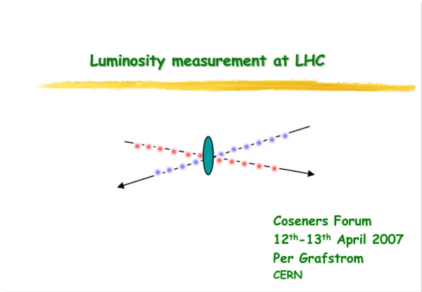
Download
1 / 31
310 likes | 438 Views
Luminosity Measurement at the International Linear Collider. Iftach Sadeh Tel Aviv University ( On behalf of the FCAL collaboration ). December 28 th 2008. http://alzt.tau.ac.il/~sadeh/ sadeh@alzt.tau.ac.il. Overview. 2. The International Linear Collider (ILC).

E N D
Luminosity Measurement at the International Linear Collider Iftach SadehTel Aviv University( On behalf of the FCAL collaboration ) December 28th 2008 http://alzt.tau.ac.il/~sadeh/sadeh@alzt.tau.ac.il
Overview 2 The International Linear Collider (ILC). Luminosity measurement at the ILC. Design and performance of the luminosity calorimeter (LumiCal). A clustering algorithm for LumiCal.
The ILC & The ILD detector 3 LumiCal
LumiCal Performance requirements Compare angles & energy X,Y RIGHT θ Z 4 • Required precision is: • Measure luminosity by counting the number of Bhabha events (NB) in a well defined angular and energetic range:
LumiCal Design parameters 5 • 1. Placement: • 2270 mm from the IP • Inner Radius - 80 mm • Outer Radius - 190 mm 2. Segmentation: • 48 azimuthal & 64 radial divisions: • Azimuthal Cell Size - 131 mrad • Radial Cell Size - 0.8 mrad 3. Layers: • Number of layers - 30 • Tungsten Thickness - 3.5 mm • Silicon Thickness - 0.3 mm • Elec. Space - 0.1 mm • Support Thickness - 0.6 mm
ares Intrinsic parameters of LumiCal σ(θ) • Position reconstruction (polar angle): 6 • Relative energy resolution: Logarithmic constant (C) Bias Resolution
Topology of Bhabha scattering 7 • Bhabha scattering with √s = 500 GeV • Separation between photons and leptons, as a function of the energy of the low-energy-particle. θ Φ Energy
Clustering Algorithm 8 • Phase I:Near-neighbor clustering in a single layer. • Phase II:Cluster-merging in a single layer. • Phase III:Global (multi-layer) clustering.
Overlap of multiple showers 9 • Profile of the energy of a single 250 GeV shower. • Profile of the energy of two showers (230 and 20 GeV) separated by one Moliere radius (indicated by the circles).
Clustering - Results (event-by-event) 10 (EGen- ERec)/ EGen • Event-by-event comparison of the energy and position of showers (GEN) and clusters (REC) as a function ofEGen. (ΦGen- ΦRec)/ ΦGen (θGen- θRec)/ θGen
Summary 11 • Intrinsic properties of LumiCal: • Energy resolution: ares ≈ 0.21 √GeV. • Relative error in the luminosity measurement:ΔL/L = e(rec) e(stat) = 1.5 · 10-4 4 · 10-5 (at 500 fb-1). • The reconstruction error, e(rec), is due to the error in reconstruction of the polar angle. • The statistical error, e(stat), is due to fluctuations in the expected number of Bhabha events, ΔNB/NB, for an integrated luminosity of 500 fb-1. • The theoretical uncertainty is expected to be ~ 2 · 10-4. • Partial event reconstruction (counting of radiative photons): • Merging-cuts need to be made on the minimal energy of a cluster and on the separation between any pair of clusters. • The algorithm performs with high efficiency and purity. The number of radiative photons within a well defined phase-space may be counted with an acceptable uncertainty.
Physics Background leptonic Four-fermion processes hadronic 14 • Four-fermion processes are the main background, dominated by two-photon events (bottom right diagram). BEFORE AFTER cut The cuts reduce the background to the level of 10-4
Selection of Bhabha events Simulation distribution Distribution after acceptance and energy balance selection Left side signal Compare angles & energy X,Y RIGHT θ Z Right side signal 15 Acoplanarity Acolinearity Energy Balance
Detector signal σ(θ) ares 16 • Distribution of the deposited energy spectrum of a MIP (using 250 GeV muons):MPV of distribution = 89 keV ~ 3.9 fC. • Distributions of the charge in a single cell for 250 GeV electron showers. • The influence of digitization on the energy resolution and on the polar bias. MIPs Digitization Signal distribution
Digitization ares σ(θ) Δθ
Thickness of the tungsten layers (dlayer) 18 ares Signal distribution Δθ σ(θ)
Number of radial divisions 19 Δθ σ(θ) • Dependence of the polar resolution, bias and subsequent error in the luminosity measurement on the angular cell-size, lθ.
Inner and outer radii 20 antiDID DID • Beamstrahlung spectrum on the face of LumiCal (14 mrad crossing angle): For the antiDID case Rmin must be larger than 7cm. 6cm 8cm 19cm
MIP (muon) Detection in LumiCal 21 • Many physics studies demand the ability to detect muons (or the lack thereof) in the Forward Region. • Example: Discrimination between super-symmetry (SUSY) and the universal extra dimensions (UED) theories may be done by measuring the smuon-pair production process. The observable in the figure, θμ, denotes the scattering angle of the two final state muons. “Contrasting Supersymmetry and Universal Extra Dimensions at Colliders” – M. Battaglia et al. (http://arxiv.org/pdf/hep-ph/0507284)
MIP (muon) Detection in LumiCal 22 • Multiple hits for the same radius (non-zero cell size). • After averaging and fitting, an extrapolation to the IP (z = 0) can be made.
Beam-Beam effects at the ILC 23 High beam-beam field (~kT) results in energy loss in the form of synchrotron radiation (beamstrahlung). Bunches are deformed by electromagnetic attraction: each beam acting as a focusing lens on the other. Change in the final state polar angle due to deflection by the opposite bunch, as a function of the production polar angle. • Since the beamstrahlung emissions occur asymmetrically between e+ and e-, the acolinearity is increased resulting in a bias in the counting rate. “Impact of beam-beam effects on precision luminosity measurements at the ILC” – C. Rimbaultet al. (http://www.iop.org/EJ/abstract/1748-0221/2/09/P09001/)
Effective layer-radius, reff(l) & Moliere Radius, RM 24 • Dependence of the layer-radius, r(l), on the layer number, l. • Distribution of the Moliere radius, RM. r(l) RM
Clustering - Algorithm 25 • Longitudinal shower shape. • Phase I:Near-neighbor clustering in a single layer. • Phase II:Cluster-merging in a single layer.
Clustering Algorithm 26 • Phase III:Global (multi-layer) clustering.
Clustering - Energy density corrections 27 • Event-by-event comparison of the energy of showers (GEN) and clusters (REC). Before After
Clustering - Results 28 • (2→1): Two showers were merged into one cluster. • (1→2): One shower was split into two clusters. • The Moliere radius is RM (= 14mm), dpair is the distance between a pair of showers, and Elow is the energy of the low-energy shower.
Clustering - Geometry dependence 29 96 div 48 div 24 div
Clustering - Results (measurable distributions) 30 • Merging-cuts:Elow ≥ 20 GeV , dpair ≥ RM Energylow Energyhigh θhigh θlow Δθhigh,low • Energy and polar angle (θ) of high and low-energy clusters/showers. • Difference in θ between the high and low-energy clusters/showers.
Clustering - Results (relative errors) 31 • Dependence on the merging-cuts of the errors in counting the number of single showers which were reconstructed as two clusters (N1→2), and the number of showers pairs which were reconstructed as single clusters, (N2→1).