Download

1 / 52
520 likes | 525 Views
Spatial Indexing I. Point Access Methods. Many slides are based on slides provided by Prof. Christos Faloutsos (CMU) and Prof. Evimaria Terzi (BU). The problem. Given a point set and a rectangular query, find the points enclosed in the query We allow insertions/deletions on line. Query.

E N D
Spatial Indexing I Point Access Methods Many slides are based on slides provided by Prof. Christos Faloutsos (CMU) and Prof. Evimaria Terzi (BU)
The problem • Given a point set and a rectangular query, find the points enclosed in the query • We allow insertions/deletions on line Query
Grid File • Hashing methods for multidimensional points (extension of Extensible hashing) • Idea: Use a grid to partition the space each cell is associated with one page • Two disk access principle (exact match)
Grid File • Start with one bucket for the whole space. • Select dividers along each dimension. Partition space into cells • Dividers cut all the way.
Grid File • Each cell corresponds to 1 disk page. • Many cells can point to the same page. • Cell directory potentially exponential in the number of dimensions
Grid File Implementation • Dynamic structure using a grid directory • Grid array: a 2 dimensional array with pointers to buckets (this array can be large, disk resident) G(0,…, nx-1, 0, …, ny-1) • Linear scales: Two 1 dimensional arrays that used to access the grid array (main memory) X(0, …, nx-1), Y(0, …, ny-1)
Example Buckets/Disk Blocks Grid Directory Linear scale Y Linear scale X
Grid File Search • Exact Match Search: at most 2 I/Os assuming linear scales fit in memory. • First use liner scales to determine the index into the cell directory • access the cell directory to retrieve the bucket address (may cause 1 I/O if cell directory does not fit in memory) • access the appropriate bucket (1 I/O) • Range Queries: • use linear scales to determine the index into the cell directory. • Access the cell directory to retrieve the bucket addresses of buckets to visit. • Access the buckets.
Grid File Insertions • Determine the bucket into which insertion must occur. • If space in bucket, insert. • Else, split bucket • how to choose a good dimension to split? • If bucket split causes a cell directory to split do so and adjust linear scales. • insertion of these new entries potentially requires a complete reorganization of the cell directory--- expensive!!!
Grid File Deletions • Deletions may decrease the space utilization. Merge buckets • We need to decide which cells to merge and a merging threshold • Buddy system and neighbor system • A bucket can merge with only one buddy in each dimension • Merge adjacent regions if the result is a rectangle
Tree-based PAMs • Most of tb-PAMs are based on kd-tree • kd-tree is a main memory binary tree for indexing k-dimensional points • Needs to be adapted for the disk model • Levels rotate among the dimensions, partitioning the space based on a value for that dimension • kd-tree is not necessarily balanced
2-dimensional kd-trees • A data structure to support range queries in R2 • Not the most efficient solution in theory • Everyone uses it in practice • Preprocessing time: O(nlogn) • Space complexity: O(n) • Query time: O(n1/2+k)
2-dimensional kd-trees • Algorithm: • Choose x or y coordinate (alternate) • Choose the median of the coordinate; this defines a horizontal or vertical line • Recurse on both sides • We get a binary tree: • Size O(n) • Depth O(logn) • Construction time O(nlogn)
Region of node v Region(v) : the subtree rooted at vstores the points in black dots
Searching in kd-trees • Range-searching in 2-d • Given a set of n points, build a data structure that for any query rectangle R reports all point in R
kd-tree: range queries • Recursive procedure starting from v = root • Search (v,R) • If v is a leaf, then report the point stored in v if it lies in R • Otherwise, if Reg(v) is contained in R, report all points in the subtree(v) • Otherwise: • If Reg(left(v)) intersects R, then Search(left(v),R) • If Reg(right(v)) intersects R, then Search(right(v),R)
Query time analysis • We will show that Searchtakes at most O(n1/2+P) time, where P is the number of reported points • The total time needed to report all points in all sub-trees is O(P) • We just need to bound the number of nodes v such that region(v) intersects R but is not contained in R (i.e., boundary of R intersects the boundary of region(v)) • gross overestimation: bound the number of region(v) which are crossed by any of the 4 horizontal/vertical lines
Query time (Cont’d) • Q(n): max number of regions in an n-point kd-tree intersecting a (say, vertical) line? • If ℓ intersects region(v) (due to vertical line splitting), then after two levels it intersects 2 regions (due to 2 vertical splitting lines) • The number of regions intersecting ℓ is Q(n)=2+2Q(n/4) Q(n)=(n1/2)
d-dimensional kd-trees • A data structure to support range queries in Rd • Preprocessing time: O(nlogn) • Space complexity: O(n) • Query time: O(n1-1/d+k)
Construction of the d-dimensional kd-trees • The construction algorithm is similar as in 2-d • At the root we split the set of points into two subsets of same size by a hyper-plane vertical to x1-axis • At the children of the root, the partition is based on the second coordinate: x2-coordinate • At depth d, we start all over again by partitioning on the first coordinate • The recursion stops until there is only one point left, which is stored as a leaf
External memory kd-trees (kdB-tree) • Pack many interior nodes (forming a subtree) into a block using BFS-traversal. • it may not be feasible to group nodes at lower level into a block productively. • Many interesting papers on how to optimally pack nodes into blocks recently published. • Similar to B-tree, tree nodes split many ways instead of two ways • insertion becomes quite complex and expensive. • No storage utilization guarantee since when a higher level node splits, the split has to be propagated all the way to leaf level resulting in many empty blocks.
LSD-tree • Local Split Decision – tree • Use kd-tree to partition the space. Each partition contains up to B points. The kd-tree is stored in main-memory. • If the kd-tree (directory) is large, we store a sub-tree on disk • Goal: the structure must remain balanced: external balancing property
LSD-tree: main points • Split strategies: • Data dependent • Distribution dependent • Paging algorithm • Two types of splits: bucket splits and internal node splits
PAMs • Point Access Methods • Multidimensional Hashing: Grid File • Exponential growth of the directory • Hierarchical methods: kd-tree based • Storing in external memory is tricky • Space Filling Curves: Z-ordering • Map points from 2-dimensions to 1-dimension. Use a B+-tree to index the 1-dimensional points
Z-ordering • Basic assumption: Finite precision in the representation of each co-ordinate, K bits (2K values) • The address space is a square (image) and represented as a 2K x 2K array • Each element is called a pixel
Z-ordering • Impose a linear ordering on the pixels of the image 1 dimensional problem A ZA = shuffle(xA, yA) = shuffle(“01”, “11”) 11 = 0111 = (7)10 10 ZB = shuffle(“01”, “01”) = 0011 01 00 00 01 10 11 B
Z-ordering • Given a point (x, y) and the precision K find the pixel for the point and then compute the z-value • Given a set of points, use a B+-tree to index the z-values • A range (rectangular) query in 2-d is mapped to a set of ranges in 1-d
Queries • Find the z-values that contained in the query and then the ranges QA QA range [4, 7] 11 QB ranges [2,3] and [8,9] 10 01 00 00 01 10 11 QB
Hilbert Curve • We want points that are close in 2d to be close in the 1d • Note that in 2d there are 4 neighbors for each point where in 1d only 2. • Z-curve has some “jumps” that we would like to avoid • Hilbert curve avoids the jumps : recursive definition
Hilbert Curve- example • It has been shown that in general Hilbert is better than the other space filling curves for retrieval [Jag90] • Hi (order-i) Hilbert curve for 2ix2i array H1 ... H(n+1) H2
Handling Regions • A region breaks into one or more pieces, each one with different z-value • Works for raster representations (pixels) • We try to minimize the number of pieces in the representation: precision/space overhead trade-off ZR1 = 0010 = (2) ZR2 = 1000 = (8) 11 10 ZG = 11 01 00 ( “11” is the common prefix) 00 01 10 11
Z-ordering for Regions • Break the space into 4 equal quadrants: level-1 blocks • Level-i block: one of the four equal quadrants of a level-(i-1) block • Pixel: level-K blocks, image level-0 block • For a level-i block: all its pixels have the same prefix up to 2i bits; the z-value of the block
Quadtree • Object is recursively divided into blocks until: • Blocks are homogeneous • Pixel level • Quadtree: ‘0’ stands for S and W ‘1’ stands for N and E SW NE SE NW 10 11 00 01 11 11 10 1001 01 1011 00 00 01 10 11
Region Quadtrees • Implementations • FL (Fixed Length) • FD (Fixed length-Depth) • VL (Variable length) • Use a B+-tree to index the z-values and answer range queries
Linear Quadtree (LQ) • Assume we use n-bits in each dimension (x,y) (so we have 2nx2n pixels) • For each object O, compute the z-values of this object: z1, z2, z3, …, zk (each value can have between 0 and 2n bits) • For each value zi we append at the end the level l of this value ( level l =log(|zi|)) • We create a value with 2n+l bits for each z-value and we insert it into a B+-tree (l= log2(h))
Z-value, l | Morton block A: 00, 01 = 00000001 B: 0110, 10 = 01100010 C: 111000,11 = 11100011 n=3 A:1, B:98, C: 227 Insert into B+-tree using Mb B C A
Query Alg WindowQ(query w, quadtree block b) { Mb = Morton block of b; If b is totally enclosed in w { Compute Mbmax Use B+-tree to find all objects with M values between Mb<=M<= Mbmax add to result } else { Find all objects with Mb in the B+-tree add to result Decompose b into four quadrants sw, nw, se, ne For child in {sw, nw, se, ne} if child overlaps with w WindowQ(w, child) } }
z-ordering - analysis Q: How many pieces (‘quad-tree blocks’) per region? A: proportional to perimeter (surface etc)
z-ordering - analysis (How long is the coastline, say, of Britain? Paradox: The answer changes with the yard-stick -> fractals ...) http://en.wikipedia.org/wiki/How_Long_Is_the_Coast_of_Britain%3F_Statistical_Self-Similarity_and_Fractional_Dimension
Unit: 200 km, 100 km and 50 km in length. The resulting coastline is about 2350 km, 2775 km and 3425 km https://commons.wikimedia.org/wiki/File:Britain-fractal-coastline-50km.png#/media/File:Britain-fractal-coastline-combined.jpg
z-ordering - analysis Q: Should we decompose a region to full detail (and store in B-tree)?
z-ordering - analysis Q: Should we decompose a region to full detail (and store in B-tree)? A: NO! approximation with 1-5 pieces/z-values is best [Orenstein90]
z-ordering - analysis Q: how to measure the ‘goodness’ of a curve?