Download
1 / 51
510 likes | 578 Views
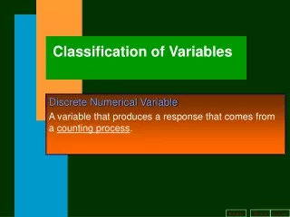
Classification of Variables. Discrete Numerical Variable A variable that produces a response that comes from a counting process. Classification of Variables. Continuous Numerical Variable A variable that produces a response that is the outcome of a measurement process.

E N D
Classification of Variables Discrete Numerical Variable A variable that produces a response that comes from a counting process.
Classification of Variables Continuous Numerical Variable A variable that produces a response that is the outcome of a measurement process.
Classification of Variables Categorical Variables Variables that produce responses that belong to groups (sometimes called “classes”) or categories.
Measurement Levels Nominal and Ordinal Levels of Measurement refer to data obtained from categorical questions. • A nominal scale indicates assignments to groups or classes. • Ordinal data indicate rank ordering of items.
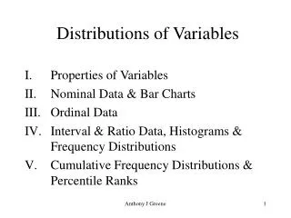
Frequency Distributions A frequency distribution is a table used to organize data. The left column (called classes or groups) includes numerical intervals on a variable being studied. The right column is a list of the frequencies, or number of observations, for each class. Intervals are normally of equal size, must cover the range of the sample observations, and be non-overlapping.
Construction of a Frequency Distribution • Rule 1: Intervals (classes) must be inclusive and non-overlapping; • Rule 2: Determine k, the number of classes; • Rule 3: Intervals should be the same width, w; the width is determined by the following: Both k and w should be rounded upward, possibly to the next largest integer.
Construction of a Frequency Distribution Quick Guide to Number of Classes for a Frequency Distribution Sample Size Number of Classes Fewer than 50 5 – 6 classes 50 to 100 6 – 8 classes over 100 8 – 10 classes
Cumulative Frequency Distributions A cumulative frequency distribution contains the number of observations whose values are less than the upper limit of each interval. It is constructed by adding the frequencies of all frequency distribution intervals up to and including the present interval.
Relative Cumulative Frequency Distributions A relative cumulative frequency distributionconverts all cumulative frequencies to cumulative percentages
Histograms and Ogives A histogram is a bar graph that consists of vertical bars constructed on a horizontal line that is marked off with intervals for the variable being displayed. The intervals correspond to those in a frequency distribution table. The height of each bar is proportional to the number of observations in that interval.
Histograms and Ogives An ogive, sometimes called a cumulative line graph, is a line that connects points that are the cumulative percentage of observations below the upper limit of each class in a cumulative frequency distribution.
Stem-and-Leaf Display A stem-and-leaf display is an exploratory data analysis graph that is an alternative to the histogram. Data are grouped according to their leading digits (called the stem) while listing the final digits (called leaves) separately for each member of a class. The leaves are displayed individually in ascending order after each of the stems.
Stem-and-Leaf Display Stem-and-Leaf Display for Gilotti’s Deli Example
Tables- Bar and Pie Charts - Frequency and Relative Frequency Distribution for Top Company Employers Example
Tables- Bar and Pie Charts - Figure 2.9 Bar Chart for Top Company Employers Example
Tables- Bar and Pie Charts - Figure 2.10 Pie Chart for Top Company Employers Example
Pareto Diagrams A Pareto diagramis a bar chart that displays the frequency of defect causes. The bar at the left indicates the most frequent cause and bars to the right indicate causes in decreasing frequency. A Pareto diagram is use to separate the “vital few” from the “trivial many.”
Line Charts A line chart, also called atime plot, is a series of data plotted at various time intervals. Measuring time along the horizontal axis and the numerical quantity of interest along the vertical axis yields a point on the graph for each observation. Joining points adjacent in time by straight lines produces a time plot.
Parameters and Statistics A statistic is a descriptive measure computed from a sample of data. A parameteris a descriptive measure computed from an entire population of data.
Measures of Central Tendency- Arithmetic Mean - The arithmetic meanof a set of data is the sum of the data values divided by the number of observations.
Sample Mean If the data set is from a sample, then the sample mean, , is:
Population Mean If the data set is from a population, then the population mean, , is:
Measures of Central Tendency- Median - An ordered arrayis an arrangement of data in either ascending or descending order. Once the data are arranged in ascending order, the median is the value such that 50% of the observations are smaller and 50% of the observations are larger.
Measures of Central Tendency- Median - If the sample size n is an odd number, the median, Xm, is the middle observation. If the sample size n is an even number, the median, Xm, is the average of the two middle observations. The median will be located in the 0.50(n+1)th ordered position.
Measures of Central Tendency- Mode - The mode, if one exists, is the most frequently occurring observation in the sample or population.
Shape of the Distribution The shape of the distribution is said to be symmetric if the observations are balanced, or evenly distributed, about the mean. In a symmetric distribution the mean and median are equal.
Shape of the Distribution A distribution isskewed if the observations are not symmetrically distributed above and below the mean. A positively skewed (or skewed to the right) distribution has a tail that extends to the right in the direction of positive values. A negatively skewed (or skewed to the left) distribution has a tail that extends to the left in the direction of negative values.
Measures of Central Tendency - Geometric Mean - The Geometric Meanis the nth root of the product of n numbers: The Geometric Mean is used to obtain mean growth over several periods given compounded growth from each period.
Measures of Variability- The Range - The rangeis in a set of data is the difference between the largest and smallest observations
Measures of Variability- Sample Variance - The sample variance, s2,is the sum of the squared differences between each observation and the sample mean divided by the sample size minus 1.
Measures of Variability- Short-cut Formulas for s2 Short-cut formulas for the sample variance, s2,are:
Measures of Variability- Population Variance - The population variance, 2, is the sum of the squared differences between each observation and the population mean divided by the population size, N.
Measures of Variability- Sample Standard Deviation - The sample standard deviation, s,is the positive square root of the variance, and is defined as:
Measures of Variability- Population Standard Deviation- The population standard deviation, ,is
The Empirical Rule(the 68%, 95%, or almost all rule) For a set of data with a mound-shaped histogram, the Empirical Rule is: • approximately 68% of the observations are contained with a distance of one standard deviation around the mean; 1 • approximately 95% of the observations are contained with a distance of 2 standard deviations around the mean; 2 • almost all of the observations are contained with a distance of three standard deviation around the mean; 3
Coefficient of Variation The Coefficient of Variation, CV,is a measure of relative dispersion that expresses the standard deviation as a percentage of the mean (provided the mean is positive). The sample coefficient of variation is
Coefficient of Variation The population coefficient of variation is
Percentiles and Quartiles Data must first be in ascending order. Percentiles separate large ordered data sets into 100ths. The Pth percentile is a number such that P percent of all the observations are at or below that number. Quartiles are descriptive measures that separate large ordered data sets into four quarters.
Percentiles and Quartiles The first quartile, Q1, is another name for the 25th percentile. The first quartile divides the ordered data such that 25% of the observations are at or below this value. Q1 is located in the .25(n+1)st position when the data is in ascending order. That is,
Percentiles and Quartiles The third quartile, Q3, is another name for the 75th percentile. The first quartile divides the ordered data such that 75% of the observations are at or below this value. Q3 is located in the .75(n+1)st position when the data is in ascending order. That is,
Interquartile Range TheInterquartile Range (IQR) measures the spread in the middle 50% of the data; that is the difference between the observations at the 25th and the 75th percentiles:
Five-Number Summary TheFive-Number Summaryrefers to the five descriptive measures: minimum, first quartile, median, third quartile, and the maximum.
Box-and-Whisker Plots ABox-and-Whisker Plotis a graphical procedure that uses the Five-Number summary. A Box-and-Whisker Plot consists of an inner box that shows the numbers which span the range from Q1 Box-and-Whisker Plot to Q3. a line drawn through the box at the median. The “whiskers” are lines drawn from Q1 to the minimum vale, and from Q3 to the maximum value.
Grouped Data Mean For a population of N observations the mean is Where the data set contains observation values m1, m2, . . ., mk occurring with frequencies f1, f2, . . . fK respectively
Grouped Data Mean For a sample of n observations, the mean is Where the data set contains observation values m1, m2, . . ., mk occurring with frequencies f1, f2, . . . fK respectively
Grouped Data Variance For a population of N observations the variance is Where the data set contains observation values m1, m2, . . ., mk occurring with frequencies f1, f2, . . . fK respectively