Download
1 / 78
790 likes | 921 Views
C. E. N. T. E. R. F. O. R. I. N. T. E. G. R. A. T. I. V. E. B. I. O. I. N. F. O. R. M. A. T. I. C. S. V. U. Introduction to bioinformatics 2008 Lecture 11. Multiple Sequence Alignment benchmarking, pattern recognition and Phylogeny.

E N D
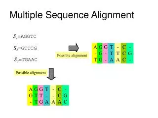
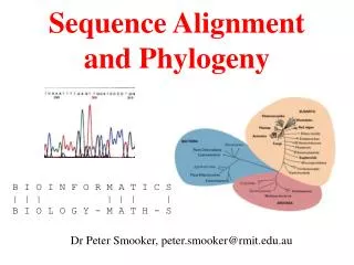
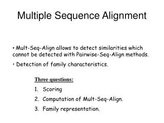
C E N T E R F O R I N T E G R A T I V E B I O I N F O R M A T I C S V U Introduction to bioinformatics 2008Lecture 11 Multiple Sequence Alignment benchmarking, pattern recognition and Phylogeny
Evaluating multiple alignments • There are reference databases based on structural information: e.g. BAliBASE and HOMSTRAD • Conflicting standards of truth • evolution • structure • function • With orphan sequences no additional information • Benchmarks depending on reference alignments • Quality issue of available reference alignment databases • Different ways to quantify agreement with reference alignment (sum-of-pairs, column score) • “Charlie Chaplin” problem
Evaluating multiple alignments • As a standard of truth, often a reference alignment based on structural superpositioning is taken These superpositionings can be scored using the root-mean-square-deviation (RMSD) of atoms that are equivalenced (taken as corresponding) in a pair of protein structures. Typically, C atoms only are used for superpositioning (main-chain trace).
BAliBASE benchmark alignments Thompson et al. (1999) NAR 27, 2682. • 8 categories: • cat. 1 - equidistant • cat. 2 - orphan sequence • cat. 3 - 2 distant groups • cat. 4 – long overhangs • cat. 5 - long insertions/deletions • cat. 6 – repeats • cat. 7 – transmembrane proteins • cat. 8 – circular permutations
. . . BAliBASE BB11001 1aab_ref1Ref1 V1 SHORT high mobility group protein BB11002 1aboA_ref1 Ref1 V1 SHORT SH3 BB11003 1ad3_ref1 Ref1 V1 LONG aldehyde dehydrogenase BB11004 1adj_ref1 Ref1 V1 LONG histidyl-trna synthetase BB11005 1ajsA_ref1 Ref1 V1 LONG aminotransferase BB11006 1bbt3_ref1 Ref1 V1 MEDIUM foot-and-mouth disease virus BB11007 1cpt_ref1 Ref1 V1 LONG cytochrome p450 BB11008 1csy_ref1 Ref1 V1 SHORT SH2 BB11009 1dox_ref1 Ref1 V1 SHORT ferredoxin [2fe-2s]
Scoring a single MSA with the Sum-of-pairs (SP) score Good alignments should have a high SP score, but it is not always the case that the true biological alignment has the highest score. • Sum-of-Pairs score • Calculate the sum of all pairwise alignment scores • This is equivalent to taking the sum of all matched a.a. pairs • The latter can be done using gap penalties or not
Evaluation measures Query Reference Column score What fraction of the MSA columns in the reference alignment is reproduced by the computed alignment Sum-of-Pairs score What fraction of the matched amino acid pairs in the reference alignment is reproduced by the computed alignment
Evaluating multiple alignmentsCharlie Chaplin problem SP BAliBASE alignment nseq * len
Summary • Individual alignments can be scored with the SP score. • Better alignments should have better SP scores • However, there is the Charlie Chaplin problem • A test and a reference multiple alignment can be scored using the SP score or the column score (now for pairs of alignments) • Evaluations show that there is no MSA method that always wins over others in terms of alignment quality
C E N T E R F O R I N T E G R A T I V E B I O I N F O R M A T I C S V U Introduction to bioinformatics 2008 Pattern Recognition
PatternsSome are easy some are not • Knitting patterns • Cooking recipes • Pictures (dot plots) • Colour patterns • Maps In 2D and 3D humans are hard to be beat by a computational pattern recognition technique, but humans are not so consistent
Example of algorithm reuse: Data clustering • Many biological data analysis problems can be formulated as clustering problems • microarray gene expression data analysis • identification of regulatory binding sites (similarly, splice junction sites, translation start sites, ......) • (yeast) two-hybrid data analysis (experimental technique for inference of protein complexes) • phylogenetic tree clustering (for inference of horizontally transferred genes) • protein domain identification • identification of structural motifs • prediction reliability assessment of protein structures • NMR peak assignments • ......
Data Clustering Problems • Clustering: partition a data set into clusters so thatdata points of the same cluster are “similar” and points of different clusters are “dissimilar” • Cluster identification-- identifying clusters with significantly different features than the background
Application Examples • Regulatory binding site identification: CRP (CAP) binding site • Two hybrid data analysis • Gene expression data analysis These problems are all solvable by a clustering algorithm
Multivariate statistics – Cluster analysis C1 C2 C3 C4 C5 C6 .. 1 2 3 4 5 Raw table Any set of numbers per column • Multi-dimensional problems • Objects can be viewed as a cloud of points in a multidimensional space • Need ways to group the data
Multivariate statistics – Cluster analysis C1 C2 C3 C4 C5 C6 .. 1 2 3 4 5 Raw table Any set of numbers per column Similarity criterion Similarity matrix Scores 5×5 Cluster criterion Dendrogram
Comparing sequences - Similarity Score - • Many properties can be used: • Nucleotide or amino acid composition • Isoelectric point • Molecular weight • Morphological characters • But: molecular evolution through sequence alignment
Multivariate statistics – Cluster analysis Now for sequences 1 2 3 4 5 Multiple sequence alignment Similarity criterion Similarity matrix Scores 5×5 Cluster criterion Phylogenetic tree
Human -KITVVGVGAVGMACAISILMKDLADELALVDVIEDKLKGEMMDLQHGSLFLRTPKIVSGKDYNVTANSKLVIITAGARQ Chicken -KISVVGVGAVGMACAISILMKDLADELTLVDVVEDKLKGEMMDLQHGSLFLKTPKITSGKDYSVTAHSKLVIVTAGARQ Dogfish –KITVVGVGAVGMACAISILMKDLADEVALVDVMEDKLKGEMMDLQHGSLFLHTAKIVSGKDYSVSAGSKLVVITAGARQ Lamprey SKVTIVGVGQVGMAAAISVLLRDLADELALVDVVEDRLKGEMMDLLHGSLFLKTAKIVADKDYSVTAGSRLVVVTAGARQ Barley TKISVIGAGNVGMAIAQTILTQNLADEIALVDALPDKLRGEALDLQHAAAFLPRVRI-SGTDAAVTKNSDLVIVTAGARQ Maizey casei -KVILVGDGAVGSSYAYAMVLQGIAQEIGIVDIFKDKTKGDAIDLSNALPFTSPKKIYSA-EYSDAKDADLVVITAGAPQ Bacillus TKVSVIGAGNVGMAIAQTILTRDLADEIALVDAVPDKLRGEMLDLQHAAAFLPRTRLVSGTDMSVTRGSDLVIVTAGARQ Lacto__ste -RVVVIGAGFVGASYVFALMNQGIADEIVLIDANESKAIGDAMDFNHGKVFAPKPVDIWHGDYDDCRDADLVVICAGANQ Lacto_plant QKVVLVGDGAVGSSYAFAMAQQGIAEEFVIVDVVKDRTKGDALDLEDAQAFTAPKKIYSG-EYSDCKDADLVVITAGAPQ Therma_mari MKIGIVGLGRVGSSTAFALLMKGFAREMVLIDVDKKRAEGDALDLIHGTPFTRRANIYAG-DYADLKGSDVVIVAAGVPQ Bifido -KLAVIGAGAVGSTLAFAAAQRGIAREIVLEDIAKERVEAEVLDMQHGSSFYPTVSIDGSDDPEICRDADMVVITAGPRQ Thermus_aqua MKVGIVGSGFVGSATAYALVLQGVAREVVLVDLDRKLAQAHAEDILHATPFAHPVWVRSGW-YEDLEGARVVIVAAGVAQ Mycoplasma -KIALIGAGNVGNSFLYAAMNQGLASEYGIIDINPDFADGNAFDFEDASASLPFPISVSRYEYKDLKDADFIVITAGRPQ Lactate dehydrogenase multiple alignment Distance Matrix 1 2 3 4 5 6 7 8 9 10 11 12 13 1 Human 0.000 0.112 0.128 0.202 0.378 0.346 0.530 0.551 0.512 0.524 0.528 0.635 0.637 2 Chicken 0.112 0.000 0.155 0.214 0.382 0.348 0.538 0.569 0.516 0.524 0.524 0.631 0.651 3 Dogfish 0.128 0.155 0.000 0.196 0.389 0.337 0.522 0.567 0.516 0.512 0.524 0.600 0.655 4 Lamprey 0.202 0.214 0.196 0.000 0.426 0.356 0.553 0.589 0.544 0.503 0.544 0.616 0.669 5 Barley 0.378 0.382 0.389 0.426 0.000 0.171 0.536 0.565 0.526 0.547 0.516 0.629 0.575 6 Maizey 0.346 0.348 0.337 0.356 0.171 0.000 0.557 0.563 0.538 0.555 0.518 0.643 0.587 7 Lacto_casei 0.530 0.538 0.522 0.553 0.536 0.557 0.000 0.518 0.208 0.445 0.561 0.526 0.501 8 Bacillus_stea 0.551 0.569 0.567 0.589 0.565 0.563 0.518 0.000 0.477 0.536 0.536 0.598 0.495 9 Lacto_plant 0.512 0.516 0.516 0.544 0.526 0.538 0.208 0.477 0.000 0.433 0.489 0.563 0.485 10 Therma_mari 0.524 0.524 0.512 0.503 0.547 0.555 0.445 0.536 0.433 0.000 0.532 0.405 0.598 11 Bifido 0.528 0.524 0.524 0.544 0.516 0.518 0.561 0.536 0.489 0.532 0.000 0.604 0.614 12 Thermus_aqua 0.635 0.631 0.600 0.616 0.629 0.643 0.526 0.598 0.563 0.405 0.604 0.000 0.641 13 Mycoplasma 0.637 0.651 0.655 0.669 0.575 0.587 0.501 0.495 0.485 0.598 0.614 0.641 0.000 How can you see that this is a distance matrix?
Multivariate statistics – Cluster analysis C1 C2 C3 C4 C5 C6 .. 1 2 3 4 5 Data table Similarity criterion Similarity matrix Scores 5×5 Cluster criterion Dendrogram/tree
Multivariate statistics – Cluster analysisWhy do it? • Finding a true typology • Model fitting • Prediction based on groups • Hypothesis testing • Data exploration • Data reduction • Hypothesis generation • But you can never prove a classification/typology!
Cluster analysis – data normalisation/weighting C1 C2 C3 C4 C5 C6 .. 1 2 3 4 5 Raw table Normalisation criterion C1 C2 C3 C4 C5 C6 .. 1 2 3 4 5 Normalised table Column normalisation x/max Column range normalise (x-min)/(max-min)
Cluster analysis – (dis)similarity matrix C1 C2 C3 C4 C5 C6 .. 1 2 3 4 5 Raw table Similarity criterion Similarity matrix Scores 5×5 Di,j= (k | xik – xjk|r)1/r Minkowski metrics r = 2 Euclidean distance r = 1 City block distance
(dis)similarity matrix Di,j= (k | xik – xjk|r)1/r Minkowski metrics r = 2 Euclidean distance r = 1 City block distance EXAMPLE: length height width Cow1 11 7 3 Cow 2 7 4 5 Euclidean dist. = sqrt(42 + 32 + -22) = sqrt(29) = 5.39 City Block dist. = |4|+|3|+|-2| = 9 -2 3 4
Cluster analysis – Clustering criteria Similarity matrix Scores 5×5 Cluster criterion Dendrogram (tree) Single linkage - Nearest neighbour Complete linkage – Furthest neighbour Group averaging – UPGMA Neighbour joining – global measure, used to make a Phylogenetic Tree
Cluster analysis – Clustering criteria Similarity matrix Scores 5×5 Cluster criterion Dendrogram (tree) Four different clustering criteria: Single linkage - Nearest neighbour Complete linkage – Furthest neighbour Group averaging – UPGMA Neighbour joining (global measure) Note: these are all agglomerative cluster techniques; i.e. they proceed by merging clusters as opposed to techniques that are divisive and proceed by cutting clusters
Cluster analysis – Clustering criteria • Start with N clusters of 1 object each • Apply clustering distance criterion iteratively until you have 1 cluster of N objects • Most interesting clustering somewhere in between distance Dendrogram (tree) Note: a dendrogram can be rotated along branch points (like mobile in baby room) -- distances between objects are defined along branches 1 cluster N clusters
Single linkage clustering (nearest neighbour) Char 2 Char 1
Single linkage clustering (nearest neighbour) Char 2 Char 1
Single linkage clustering (nearest neighbour) Char 2 Char 1
Single linkage clustering (nearest neighbour) Char 2 Char 1
Single linkage clustering (nearest neighbour) Char 2 Char 1
Single linkage clustering (nearest neighbour) Char 2 Char 1 Distance from point to cluster is defined as the smallest distance between that point and any point in the cluster
Single linkage clustering (nearest neighbour) Char 2 Char 1 Distance from point to cluster is defined as the smallest distance between that point and any point in the cluster
Single linkage clustering (nearest neighbour) Char 2 Char 1 Distance from point to cluster is defined as the smallest distance between that point and any point in the cluster
Single linkage clustering (nearest neighbour) Char 2 Char 1 Distance from point to cluster is defined as the smallest distance between that point and any point in the cluster
Single linkage clustering (nearest neighbour) Let Ci andCj be two disjoint clusters: di,j = Min(dp,q), where p Ci and q Cj Single linkage dendrograms typically show chaining behaviour (i.e., all the time a single object is added to existing cluster)
Complete linkage clustering (furthest neighbour) Char 2 Char 1
Complete linkage clustering (furthest neighbour) Char 2 Char 1
Complete linkage clustering (furthest neighbour) Char 2 Char 1
Complete linkage clustering (furthest neighbour) Char 2 Char 1
Complete linkage clustering (furthest neighbour) Char 2 Char 1
Complete linkage clustering (furthest neighbour) Char 2 Char 1
Complete linkage clustering (furthest neighbour) Char 2 Char 1