Download
1 / 88
920 likes | 995 Views
Explore various optimization methods in data mining, from combinatorial optimization to genetic algorithms. Understand problem formulation, algorithms, and solutions like feature selection and classification. Dive into genetic algorithms, their formulation, and applications in solving data mining problems. Learn about single-point crossover, two-point crossover, uniform crossover, and mutation in genetic algorithms for problem-solving. Access a detailed analysis of genetic algorithms, including schemas and their implications for convergence and finding solutions. Discover how genetic algorithms can be used for feature selection in data mining applications.

E N D
Overview Optimization Combinatorial Optimization Mathematical Programming Support Vector Machines Genetic Algorithm Steepest Descent Search Neural Nets, Bayesian Networks (optimize parameters) Feature selection Classification Clustering Classification, Clustering, etc
What is Optimization? Problem • Formulation • Decision variables • Objective function • Constraints • Solution • Iterative algorithm • Improving search Formulation Model Algorithm Solution
Combinatorial Optimization • Finitely many solutions to choose from • Select the best rule from a finite set of rules • Select the best subset of attributes • Too many solutions to consider all • Solutions • Branch-and-bound (better than Weka exhaustive search) • Random search
Random Search • Select an initial solution x(0) and let k=0 • Loop: • Consider the neighborsN(x(k)) of x(k) • Select a candidate x’ from N(x(0)) • Check the acceptance criterion • If accepted then let x(k+1) = x’ and otherwise let x(k+1) = x(k) • Until stopping criterion is satisfied
Common Algorithms • Simulated Annealing (SA) • Idea: accept inferior solutions with a given probability that decreases as time goes on • Tabu Search (TS) • Idea: restrict the neighborhood with a list of solutions that are tabu (that is, cannot be visited) because they were visited recently • Genetic Algorithm (GA) • Idea: neighborhoods based on ‘genetic similarity’ • Most used in data mining applications
Genetic Algorithms • Maintain a population of solutions rather than a single solution • Members of the population have certain fitness (usually just the objective) • Survival of the fittest through • selection • crossover • mutation
GA Formulation • Use binary strings (or bits) to encode solutions: 0 1 1 0 1 0 0 1 0 • Terminology • Chromosomes = solution • Parent chromosome • Children or offspring
Problems Solved • Data Mining Problems that have been addressed using Genetic Algorithms: • Classification • Attribute selection • Clustering
Classification Example Sunny 100 Overcast 010 Rainy 001 Yes 10 No 01 Outlook Windy
Representing a Rule If windy=yes then play=yes If outlook=overcast and windy=yes then play=no
Single-Point Crossover ParentsOffspring Crossover point
Two-Point Crossover ParentsOffspring Crossover points
Uniform Crossover ParentsOffspring Problem?
Mutation ParentOffspring Mutated bit
Selection • Which strings in the population should be operated on? • Rank and select the n fittest ones • Assign probabilities according to fitness and select probabilistically, say
Creating a New Population • Create a population Pnew with p individuals • Survival • Allow individuals from old population to survived intact • Rate: 1-r % of population • How to select the individuals that survive: Deterministic/random • Crossover • Select fit individuals and create new once • Rate: r% of population. How to select? • Mutation • Slightly modify any on the above individuals • Mutation rate: m • Fixed number of mutations versus probabilistic mutations
GA Algorithm • Randomly generate an initial population P • Evaluate the fitness f(xi) of each individual in P • Repeat: • Survival: Probabilistically select (1-r)p individuals from P and add to Pnew, according to • Crossover: Probabilistically select rp/2 pairs from P and apply the crossover operator. Add to Pnew • Mutation: Uniformly choose m percent of member and invert one randomly selected bit • Update: P Pnew • Evaluate: Compute the fitness f(xi) of each individual in P • Return the fittest individual from P
Analysis of GA: Schemas • Does GA converge? • Does GA move towards a good solution? Local optima? • Holland (1975): Analysis based on schemas • Schema: string combination of 0s, 1s, *s • Example: 0*10 represents {0010,0110}
The Schema Theorem(all the theory on one slide) Average fitness of individuals in schema s at time t Number of defined bits in schema s Distance between defined bits in s Probability of crossover Probability of mutation Number of instance of schema s at time t
Interpretation • Fit schemas grow in influence • What is missing • Crossover? • Mutation? • How about time t+1 ? • Other approaches: • Markov chains • Statistical mechanics
GA for Feature Selection • Feature selection: • Select a subset of attributes (features) • Reason: to many, redundant, irrelevant • Set of all subsets of attributes very large • Little structure to search • Random search methods
Encoding • Need a bit code representation • Have some n attributes • Each attribute is either in (1) or out (0) of the selected set
Fitness • Wrapper approach • Apply learning algorithm, say a decision tree, to the individual x ={outlook, humidity} • Let fitness equal error rate (minimize) • Filter approach • Let fitness equal the entropy (minimize) • Other diversity measures can also be used • Simplicity measure?
Crossover Crossover point
Clustering Example Create two clusters for: {10,20} {30,40} {10,20,40} {30} {20,40} {10,30} {20} {10,30,40} Crossover
Discussion • GA is a flexible and powerful random search methodology • Efficiency depends on how well you can encode the solutions in a way that will work with the crossover operator • In data mining, attribute selection is the most natural application
Attribute Selection in Unsupervised Learning • Attribute selection typically uses a measure, such as accuracy, that is directly related to the class attribute • How do we apply attribute selection to unsupervised learning such as clustering? • Need a measure • compactness of cluster • separation among clusters Multiple measures
Quality Measures • Compactness Instances Clusters Centroid Number of attributes Normalization constant to make
More Quality Measures • Cluster Separation
Final Quality Measures • Adjustment for bias • Compexity
Wrapper Framework • Loop: • Obtain an attribute subset • Apply k-means algorithm • Evaluate cluster quality • Until stopping criterion satisfied
Problem • What is the optimal attribute subset? • What is the optimal number of clusters? • Try to find simultaneously
Example • Find an attribute subset and optimal number of clusters (Kmin = 2, Kmin = 3) for
Formulation • Define an individual • Initial Population 0 1 0 1 1 1 0 0 1 0
Evaluate Fitness • Start with 0 1 0 1 1 • Three clusters and {Sepal Width, Petal Width} • Apply k-means with k=3
K-Means • Start with random centroids: 10, 70, 80
New Centroids No change in assignment so terminate k-means algorithm
Quality of Clusters • Centers • Center 1 at (3.46,0.34): {60,70,90,100} • Center 2 at (3.30,1.60): {80} • Center 3 at (2.73,1.28): {10,20,30,40,50} • Evaluation
Next Individual • Now look at 1 0 0 1 0 • Two clusters and {Sepal Length, Petal Width} • Apply k-means with k=3
K-Means • Say we select 20 and 90 as initial centroids:
Recalculate Again No change in assignment so terminate k-means algorithm
Quality of Clusters • Centers • Center 1 at (4.92,0.45): {10,20,30,40,50,90} • Center 3 at (6.28,1.43): {60,70,90,100} • Evaluation
Compare Individuals Which is fitter?
Evaluating Fitness • Can scale (if necessary) • Then weight them together, e.g., • Alternatively, we can use Pareto optimization
Mathematical Programming • Continuous decision variables • Constrained versus non-constrained • Form of the objective function • Linear Programming (LP) • Quadratic Programming (QP) • General Mathematical Programming (MP)
Optimal solution 10 Linear Program