Download

1 / 11
120 likes | 276 Views
Query Optimization to Data Mining. Most people have Data from which they want information. So, most people need DBMSs whether they know it or not. The main component of any DBMS is the query processor.

E N D
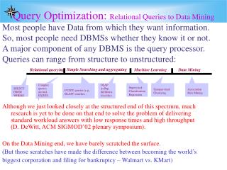
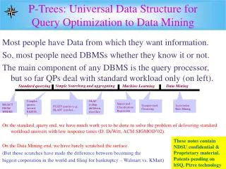
Query Optimization to Data Mining Most people have Data from which they want information. So, most people need DBMSs whether they know it or not. The main component of any DBMS is the query processor. On the standard_query end, we have much work yet to be done to solve the problem of delivering standard workload answers with low response times (D. DeWitt, ACM SIGMOD’02). On the Data Mining end, we have barely scratched the surface. (But those scratches have made the difference between becoming the biggest corporation in the world and filing for bankruptcy – Walmart vs. KMart) Simple Searching and aggregating Standard querying Machine Learning Data Mining Complex queries (nested, EXISTS..) FUZZY queries (e.g., BLAST searches, .. OLAP (rollup, drilldown, slice/dice.. Supervised - Classification Regression Unsupervised- Clustering Association Rule Mining SELECT FROM WHERE
BSM — A Bit Level Decomposition Storage ModelA model of query optimization of all types • Vertical partitioning has been studied within the context of both centralized database system as well as distributed ones. It is a good strategy when small numbers of columns are retrieved by most queries. The decomposition of a relation also permits a number of transactions to execute concurrently. Copeland et al presented an attribute level decomposition storage model (DSM) [CK85] storing each column of a relational table into a separate binary table. The DSM showed great comparability in performance. • Beyond attribute level decomposition, Wong et al further took the advantage of encoding attribute values using a small number of bits to reduce the storage space [WLO+85]. In this paper, we will decompose attributes of relational tables into bit position level, utilize SPJ query optimization strategy on them, store the query results in one relational table, finally data mine using our very good P-tree methods. • Our method offers these advantages: • (1) By vertical partitioning, we only need to read everything we need. This method makes hardware caching work really well and greatly increases the effectiveness of the I/O device. • (2) We encode attribute values into bit vector format, which makes compression easy to do. • (3) SPJ queries can be formulated as Boolean expressions, which facilitates fast implementation on hardware. • (4) Our model is fit not only for query processing but for data mining as well. • [CK85] G.Copeland, S. Khoshafian. A Decomposition Storage Model. Proc. ACM Int. Conf. on Management of Data (SIGMOD’85), pp.268-279, Austin, TX, May 1985. • [WLO+85] H. K. T. Wong, H.-F. Liu, F. Olken, D. Rotem, and L. Wong. Bit Transposed Files. • Proc. Int. Conf. on Very Large Data Bases (VLDB’85), pp.448-457, Stockholm, Sweden, 1985.
SPJ Query Optimization Strategies - One-table Selections • There are two categories of queries in one-table selections: Equality Queries and Range Queries. Most techniques [WLO+85, OQ97, CI98] used to optimize them employ encoding schemes – equality encoding and range encoding. Chan and Ioannidis [CI99] defined a more general query format called interval query. An interval query on attribute A is a query of the form “x≤A≤y” or “NOT (x≤A≤y)”. It can be an equality query or a range query when x or y satisfies different kinds of conditions. • We defined interval P-trees in previous work [DKR+02], which is equivalent to the bit vectors of corresponding intervals. So for each restriction in the form above, we have one corresponding interval P-tree. The ANDing result of all the corresponding interval P-trees represents all the rows satisfy the conjunction of all the restriction in the where clause. • [CI98] C.Y. Chan and Y. Ioannidis. Bitmap Index Design and Evaluation. Proc. ACM Intl. Conf. on Management of Data (SIGMOD’98), pp.355-366, Seattle, WA, June 1998. • [CI99] C.Y. Chan and Y.E. Ioannidis. An Efficient Bitmap Encoding Scheme for Selection Queries. Proc. ACM Intl. Conf. on Management of Data (SIGMOD’99), pp.216-226, Philadephia, PA, 1999. • [DKR+02] Q. Ding, M. Khan, A. Roy, and W. Perrizo. The P-tree algebra. Proc. ACM Symposium Applied Computing (SAC 2002), pp.426-431, Madrid, Spain, 2002. • [OQ97] P. O’Neill and D. Quass. Improved Query Performance with Variant Indexes. Proc. ACM Int. Conf. on Management of Data (SIGMOD’97), pp.38-49, Tucson, AZ, May 1997.
Select-Project-StarJoin (SPSJ) Queries A Select-Project-StarJoin query is a SPJ query in which there is one multiway join along with selections and projections typically there is a central fact relation to which several dimension relations are joined. The dimension relations can be viewed as points on a star centered on the fact relation. For example, given the Student (S), Course (C), and Enrollment (E) database shown below (note a bit encoding is shown in reduced font italics for certain attributes), take SPSJ query, SELECT S.s,S.name,C.name FROM S,C,E WHERE S.s=E.s AND C.c=E.c AND S.gen=M AND E.grade=A AND C.term=S S|s____|name_|gen| C|c____|name|st|term| E|s____|c____|grade | |0 000|CLAY |M 0| |0 000|BI |ND|F 0| |0 000|1 001|B 10| |1 001|THAIS|M 0| |1 001|DB |ND|S 1| |0 000|0 000|A 11| |2 010|GOOD |F 1| |2 010|DM |NJ|S 1| |3 011|1 001|A 11| |3 011|BAID |F 1| |3 011|DS |ND|F 0| |3 011|3 011|D 00| |4 100|PERRY|M 0| |4 100|SE |NJ|S 1| |1 001|3 011|D 00| |5 101|JOAN |F 1| |5 101|AI |ND|F 0| |1 001|0 000|B 10| |2 010|2 010|B 10| |2 010|3 011|A 11| |4 100|4 100|B 10| |5 101|5 101|B 10| The bSQ attributes are stored as follows (note, e.g., bit-1 of S.s has been labeled Ss1, etc.). Ss1 Ss2 Ss3 Sg Cc1 Cc2 Cc3 Ct Es1 Es2 Es3 Ec1 Ec2 Ec3 Eg1 Eg2 0011 0000 0101 0001 0011 0000 0101 0110 0000 0000 0011 0000 0010 1010 1101 0100 00 11 01 11 00 11 01 10 0000 1111 1100 0000 0111 1101 1011 1001 11 00 01 11 00 01 11 00 BSQ attributes stored as single attribute files: S.name C.name C.st |CLAY | |BI | |ND| |THAIS| |DB | |ND| |GOOD | |DM | |NJ| |BAID | |DS | |ND| |PERRY| |SE | |NJ| |JOAN | |AI | |ND|
For character string attributes, LZW or some other run-length compression could be used to further reduce storage requirements. The compression scheme should be chosen so that any range of offset entries can be uncompressed independently of the rest. Each of these BSQ files would require only a few pages of storage, allowing the entire BSQ file to be brought into memory whenever any portion of it is needed, thus eliminating the need for indexes and paging. A bit mask is formed for each selection as follows. The bit mask for S.gen=M is just the complement of S.g (since M has been coded as 0), therefore mS=Sg'. Similarly, mC=Ct and mE=Eg1 AND Eg2. mS mC mE 1110 0110 0100 00 10 1001 00 Logically ANDing mE into the E.s and E.c attributes, reduces E.s and E.c as follows. Es1 Es2 Es3 Ec1 Ec2 Ec3 0 0 0 0 0 0 0 0 1 1 1 0 0 0 0 1 1 1 We note that the reduced S.s and C.c attributes would need to be reduced only when S.s and C.c are not already surrogates attributes. In E, each tuple is compared with the participation masks, mS and mC to eliminate non-participating (E.s, E.c) pairs. The (E.s, E,c) pairs in binary are (000, 000), (011, 001) and (010, 011) or in decimal, (0,0), (3,1) and (2,3). The mask mS and mC reveal that S.s=0,1,4 and C.c=1,2,4 are the participating values. Therefore (3,1) and (2,3) are non-participating pairs and can be eliminated. Therefore there is but one participating (E.s, E.c) pair, namely (0, 0). Therefore to answer the query only the S.name value at offset 0 and the E.name value at offset 0 need to be retrieved. The output is (0, CLAY, BI). To review, once the basic P-trees for the join and selection attributes have been processed to remove all non-participants, only the participating BSQ values need to be accessed. The basic P-trees files for the join and selection attributes would typically be striped across a cluster of nodes so that the AND operations could be done very quickly in a parallel fashion. Our implementation on a 16 node cluster of 266 MHz Pentium computers shows that any multiway AND operation can be done in a few milliseconds.
Select-Project-Join (SPJ) Queries We deal with an example in which more than one join is required and there are more than one join attribute (bushy query tree). We organize our query trees using the "constellation" model in which one of the fact files is considered central and the others are points in a star around that central attribute. Each secondary star-point fact file can be the center of a "sub-star". We apply the selection masks first. Then we perform semi-joins from the boundary toward the central fact file. Finally we perform semi-joins back out again. The result is the full elimination of all non-participants. The following is an example of such a bushy query. Those details that are identical to the above are not repeated here. SELECT S.n,C.n,R.capacity FROM S,C,E,O,R WHERE S.s=E.s & C.c=O.c & O.o=E.o & O.r=R.r & S.gen=M & C.cred=2 & E.grade=A & R.capacity=10; In this query, O is taken as the central fact relation of the following database. S___________C___________ E_________________ O_______________ R_____________ |s |n|gen| |c |n|cred| |s |o |grade| |o |c |r | |r |capacity| |0 000|A|M 0| |0 00|B|1 01| |0 000|1 001|2 10| |0 000|0 00|0 01| |0 00|30 11| |1 001|T|M 0| |1 01|D|3 11| |0 000|0 000|3 11| |1 001|0 00|1 01| |1 01|20 10| |2 010|S|F 1| |2 10|M|3 11| |3 011|1 001|3 11| |2 010|1 01|0 00| |2 10|30 11| |3 011|B|F 1| |3 11|S|2 10| |3 011|3 011|0 00| |3 011|1 01|1 01| |3 11|10 01| |4 100|C|M 0| |1 001|3 011|0 00| |4 100|2 10|0 00| |5 101|J|F 1| |1 001|0 000|2 10| |5 101|2 10|2 10| Sn |2 010|2 010|2 10| |6 110|2 10|3 11| A |2 010|3 011|3 11| |7 111|3 11|2 10| T |4 100|4 100|2 10| S |5 101|5 101|2 10| Ss1 Ss2 Ss3 Sgen B 0011 0000 0101 0001 C Egrade1 Egrade2 Cn 00 11 01 11 J 1101 0100 Cc1 Cc2 Ccred1 Ccred2 B 1011 1001 00 01 01 11 D Es1 Es2 Es3 Eo1 Eo2 Eo3 11 00 11 01 11 10M 0000 0000 0011 0000 0010 1010 S 0000 1111 1100 0000 0111 1101 Rr1 Rr2 Rcap1 Rcap2 11 00 01 11 00 01 00 01 11 10 11 01 10 11 Oo1 Oo2 Oo3 Oc1 Oc2 Or1 Or2 0011 0000 0101 0011 0000 0001 1100 0011 1111 0101 0011 1101 0011 0110
2. Results in the following, Es1 Es2 Es3 Eo1 Eo2 Eo3 0 0 0 0 0 0 0 0 1 1 1 0 0 0 0 1 1 1 Rc1 Rc2 Cr1 Cr2 1 1 1 0 Oo1 Oo2 Oo3 Oc1 Oc2 Or1 Or2 0011 0000 0101 0011 0000 0001 1100 0011 1111 0101 0011 1101 0011 0110 1. Apply selection masks: mE mR mC 0100 00 00 1001 10 01 00 Es1 Es2 Es3 Eo1 Eo2 Eo3 0000 0000 0011 0000 0010 1010 0000 1111 1100 0000 0111 1101 11 00 01 11 00 01 Rc1 Rc2 Cr1 Cr2 11 10 01 11 10 11 11 10 Oo1 Oo2 Oo3 Oc1 Oc2 Or1 Or2 0011 0000 0101 0011 0000 0001 1100 0011 1111 0101 0011 1101 0011 0110 3. Apply join-attribute selection-masks externally to further reduce the P-trees: mS s=0,1,4 are the participants. mC c=3 is the only participant. mR r=2 is only participant 1110 00 00 00 01 10 Produces: Es1 Es2 Es3 Eo1 Eo2 Eo3 Rc1 Rc2 Cr1 Cr2 0 0 0 0 0 0 0 0 1 1 1 0 0 0 0 1 1 1 1 1 1 0 Oo1 Oo2 Oo3 Oc1 Oc2 Or1 Or2 0011 0000 0101 1 0 0011 1111 0101 1 1 1 0 4. Completing the elimination of newly discovered non-participants internally in each file, results in: Es1 Es2 Es3 Eo1 Eo2 Eo3 Rc1 Rc2 Cr1 Cr2 Oo1 Oo2 Oo3 Oc1 Oc2 Or1 Or2 0 0 0 0 0 0 1 0 1 1 1 0 1 1 1 1 1 1 0 5. Thus, s has to be 0 (000), o has to be 0 (000), c has to be 3 (11) and r has to be 2 (10). But o also has to be 7 (111). Since o cannot be both 0 and 7 there are no participants.
DISTINCT Keyword, GROUP BY Clause, ORDER BY Clause, HAVING Clause and Aggregate Operations • Duplicate elimination after a projection (SQL DISTINCT keyword) is one of the most expensive operations in query optimisation. In general, it is as expensive as the join operation. However, in our approach, it can automatically be done while forming the output tuples (since that is done in a order). While forming all output records for a particular value of the ORDER BY attribute, duplicates can be easily eliminated without the need for an expensive algorithm. • The ORDER BY and GROUP BY clauses are very commonly used in queries and can require a sorting of the output relation. However, in our approach, if the central relation is chosen to be the one with the sort attribute and the surrogation is according to the attribute order (typically the case – always the case for numeric attributes), then the final output records can be put together and aggregated in the requested order without a separate sort step at no additional cost. Aggregation operators such as COUNT, SUM, AVG, MAX, and MIN can be implemented without additional cost during the output formation step and any HAVING decision can be made as output records are being composed, as well. • If the Count aggregate is requested by itself, we note that P-trees automatically provide the full counts for any predicate with just one multiway AND operation.
The following example illustrates these points. SELECT DISTINCT C.c, R.capacity FROM S,C,E,O,R WHERE S.s=E.s AND C.c=O.c AND O.o=E.o AND O.r=R.r AND C.cred>1 AND (E.grade='B' OR E.grade='A') AND R.capacity>10 ORDER BY C.c; S___________C___________ E_________________ O_______________ R_____________ |s |n|gen| |c |n|cred| |s |o |grade| |o |c |r | |r |capacity| |0 000|A|M 0| |0 00|B|1 01| |0 000|1 001|2 10| |0 000|0 00|0 01| |0 00|30 11| |1 001|T|M 0| |1 01|D|3 11| |0 000|0 000|3 11| |1 001|0 00|1 01| |1 01|20 10| |2 010|S|F 1| |2 10|M|3 11| |3 011|1 001|3 11| |2 010|1 01|0 00| |2 10|30 11| |3 011|B|F 1| |3 11|S|2 10| |3 011|3 011|0 00| |3 011|1 01|1 01| |3 11|10 01| |4 100|C|M 0| |1 001|3 011|0 00| |4 100|2 10|0 00| |5 101|J|F 1| |1 001|0 000|2 10| |5 101|2 10|2 10| Sn |2 010|2 010|2 10| |6 110|2 10|3 11| A |2 010|3 011|3 11| |7 111|3 11|2 10| T |4 100|4 100|2 10| S |5 101|5 101|2 10| Ss1 Ss2 Ss3 Sgen B 0011 0000 0101 0001 C Egrade1 Egrade2 Cn 00 11 01 11 J 1101 0100 Cc1 Cc2 Ccred1 Ccred2 B 1011 1001 00 01 01 11 D Es1 Es2 Es3 Eo1 Eo2 Eo3 11 00 11 01 11 10M 0000 0000 0011 0000 0010 1010 S 0000 1111 1100 0000 0111 1101 Rr1 Rr2 Rcap1 Rcap2 11 00 01 11 00 01 00 01 11 10 11 01 10 11 Oo1 Oo2 Oo3 Oc1 Oc2 Or1 Or2 0011 0000 0101 0011 0000 0001 1100 0011 1111 0101 0011 1101 0011 0110 • Apply selection masks: mE =Egrade1 mR =Rcap1 mC =Ccred1 1101 11 01 1011 10 11 11
results in, Es1 Es2 Es3 Eo1 Eo2 Eo3 Rr1 Rr2 Cc1 Cc2 00 0 00 0 00 1 00 0 00 0 10 0 00 01 0 1 0 00 1 11 1 00 0 00 0 11 1 01 1 0 11 01 11 00 01 11 00 01 Semijoin (toward center), EO(on o=0,1,2,3,4,5), RO(on r=0,1,2), CO(on c=1,2,3), reduces Oo1 Oo2 Oo3 Oc1 Oc2 Or1 Or2 0011 0000 0101 0011 0000 0001 1100 0011 1111 0101 0011 1101 0011 0110 to Oo1 Oo2 Oo3 Oc1 Oc2 Or1 Or2 11 00 01 11 00 01 00 00 11 01 00 11 00 01 Thus, the participants are c=1,2; r=0,1,2; o=2,3,4,5. Semijoining back again produces the following. Cc1 Cc2 Rr1 Rr2 Es1 Es2 Es3 Eo1 Eo2 Eo3 0 1 00 01 00 11 00 00 11 01 1 0 1 0 11 00 01 11 00 01 Thus, s partic are s=2,4,5. Ss1 Ss2 Ss3 11 00 01 0 1 0 Output tuples are determined from participating O.c P-trees.RC(PO.c(2)) = RC(Oc1^Oc2’)=2, since Oc1 ^ Oc2’ 11 11 = 11 00 00 00Since the 1-bits are in positions 4 and 5, the two O-tuples have O.o surrogate values 4 and 5. The r-values at positions 4 and 5 of O.r are 0 and 2. Thus, we retrieve the R.capacity values at offsets 0 and 2. However, both of these R.capacity values are 30. Thus, this duplication is discovered without sorting or additional processing. The only output is (2,30). Similarly, RCntPO.c(1) = RCntOc1’^Oc2=2, Oc1’ ^ Oc2 00 00 = 00 11 11 11 Finally note, if ORDER BY clause is over an attribute which is not in the relation O (e.g., over student number, s) then we center the query tree (or wheel) on a fact file that contains the ORDER BY attribute (e.g., on E in this case). If the ORDER BY attribute is not in any fact file (in a dimension file only) then the final query tree can be re-arranged to center on the dimension file containing that attribute. Since output ordering and duplicate elimination are traditionally very expensive sub-operations of SPJ query processing, the fact that our BDM model and the P-tree data structure provide a fast and efficient way to accomplish these operations is a very favorable aspect of the approach.
Combining Data Mining and Query Processing • Many data mining request involve pre-selection, pre-join, and pre-projection of a database to isolate the specific data subset to which the data mining algorithm is to be applied. For example, in the above database, one might be interested in all Association Rules of a given support threshold and confidence threshold across all the relations of the database. The brute force way to do this is to first join all relations into one universal relation and then to mine that gigantic relation. This is not a feasible solution in most cases due to the size of the resulting universal relation. Furthermore, often some selection on that universal relation is desirable prior to the mining step. • Our approach accommodates combinations of querying and data mining without necessitation the creation of a massive universal relation as an intermediate step. Essentially, the full vertical partitioning and P-trees provide a selection and join path which can be combined with the data mining algorithm to produce the desired solution without extensive processing and massive space requirements. The collection of P-trees and BSQ files constitute a lossless, compressed version of the universal relation. Therefore the above techniques, when combined with the required data mining algorithm can produce the combination result very efficiently and directly.