Download
1 / 28
280 likes | 352 Views
Graviton Emission in The Bulk from a Higher Dimensional Black Hole. in collaboration with S. Creek , P. Kanti , K. Tamvakis hep-th/0601126. Plan of the talk :. Brief introduction to the brane world scenario

E N D
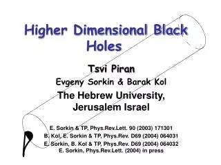
Graviton Emission in The Bulk from a Higher Dimensional Black Hole in collaboration with S. Creek , P. Kanti , K. Tamvakis hep-th/0601126
Plan of the talk: • Brief introduction to the brane world scenario • Write down the equations for graviton emission through Hawking radiation from a Schwarzschild-like black hole in the presence of extra dimensions • Solve the equations – compute energy rates for the emission • Conclusions
Introduction According to the Brane-World scenario : • SM particles confined in a 4-dimensional Brane • Gravity propagates on (4+n) dimensions (Bulk). Extra dimensions: compact, spacelike • Hierarchy problem can be solved • Black holes can be produced in colliders or in cosmic ray interactions
In the last few years there has been considerable interest in theoretical studies of these higher dimensional black holes that may be created in near future experiments (perhaps even LHC) . One important property of them : Hawking Radiation → Black holes are not completely black! → They emit radiation in a thermalspectrum , characterized by a temperature TH , such as a blackbody. → They deviate from the blackbody radiation by a factor called greybody factor. For a spherically symmetric BH
Because of the curved geometry outside a BH : some of the particles created outside the horizon will backscatter into the BH • Greybody factor measures the probability of particle escaping to infinity • Depends on particles energy, spin, angular momentum and on space dimensionality AND HAS BEEN PROVEN TO BE PROPORTIONAL TO THE INCOMING ABSORPTION PROBABILITY!
In the simplest case, that of higher dimensional Schwarzschild black holes, there have been both analytical and numerical studies for the case of Standard Model particle radiation. For example see : P. Kanti hep-ph/0402168 C.Harris ,P. Kanti hep-ph/0309054
But until recently, there have been little studies for the case of graviton emission in the bulk ! Gravitons emitted from a black hole : • will “see” the entire (4+n) dimensional space-time (Bulk) • will account for an energy loss from the brane where the BH is located, to the bulk • their emission rate will depend from the dimensionality of space-time, namely n
Our plan : ↓ ↓
FRAMEWORK:Higher Dimensional Schwarzschild BH • line element (R. Myers, M. Perry): with and dΩ2n+2 the line element in a (n+2) dimensional unit sphere The temperature of the black hole associated with Hawking radiation is
1. The equations The equations for graviton emission from a Schwarzschild BH in (4+n) dimensions are known • H. Kodama, A. Ishibashi hep-th/0305147 How to produce them : → perturb the metric outside a BH , use Einstein equations → we get 3 independent wave equations describing emitted gravitational waves , analyzed in terms of partial waves with specific angular momentum.These equations are called • Scalar perturbation equation • Vector >> • Tensor >> They describe the emitted gravitons that correspond to each type of metric perturbation. All three can be written in the form of a master equation for the partial waves
With V having different form for every perturbation. For the case of tensor and vector type we have: With l being the angular momentum quantum number and k= -1 (3) for tensor (vector) type . For the Scalar case the potential V is a bit more complicated
2. Solving the equations We will use an approximate method, valid at the low energy limit of the equations. What we will do is: • Solve the equations close to the horizon rH • Solve the equations far away from the horizon • Stretch the two solutions and match them in the intermediate zone
Boundary condition “Nothing can escape from the black hole after it crosses the horizon” So in the solution we will have we must impose the condition there are no outgoing waves in the limit r→ rH
A. Tensor and Vector type We will first look for the near horizon solution . We change the variables from r→f (r) = 1 - (rH / r) n+1 ,and after making the field redefinition and taking the limit r→rH ,the equation can be brought to the following form for the following choice for the parameters : This equations has known solutions, the hypergeometric functions
So the near horizon solution for tensor-vector mode gravitons is : With F the hypergeometric function and A1,A2 constants. By expanding this solution in the limit r→ rH and taking the boundary condition we get A2=0 We then solve the equation in the far field regime , that is far away from the horizon . The solution after taking r>>rH is easily obtained in terms of the Bessel functions : We now have to match the two solutions in the intermediate zone
We take the limit r>>rH in the near horizon solution • We take the limit ωr<<1 in the far field solution • We look in the low energy regime ωrH<<1 we compute the relation between the constants B1 , B2 We construct a solution for the whole domain of r , valid for low energies
We want the absorption probability ,so we expand the FF solution for r→ in terms of ingoing/outgoing spherical waves, and we only need to compute the ratio of their amplitudes . The result put in a compact form, is: • the same formula holds for the scalar type as well • the only dependence from the type of perturbation is in G , which is different for every type
3. Energy emission rates State multiplicities : there is a number of states that correspond to the same angular momentum number ℓ . → it depends on ℓ , n This has been computed in the literature for every type of perturbation (Rubin&Ordonez J. Math. Phys 26,65(1985)
We are finally ready to compute the energy emission rate ! Putting everything together we have We can now plot the above emission rate for all 3 types, and for every n .
Results • Vector mode gravitons are the dominant graviton mode to be emitted by the BH for every value of n • Relative magnitude of the emission rate for scalar and tensor mode gravitons depends on n • Energy emission rate in the bulk decreases as n increases, although we would expect the opposite
Conclusions • We studied graviton emission in the bulk from a spherically symmetric (4+n) dimensional Schwarzschild BH • The differential equations for the graviton emission were analytically solved for low energies using a matching technique • The equation solutions were found in the “near horizon” and “far field” regime and were stretched and matched in the intermediate zone
We thus computed the absorption probability for all 3 types of perturbations , and written down the equations describing the BH’s Hawking radiation spectrum . • We computed the energy emission rate for low energy gravitons in the bulk , which encodes information about the number of extra dimensions that might exist in nature