Download
1 / 36
360 likes | 464 Views
Visualizing Agrach ë v’s curvature of optimal control. Matthias Kawski and Eric Gehrig Arizona State University Tempe, U.S.A. This work was partially supported by NSF grant DMS 00-72369. Outline. Motivation of this work

E N D
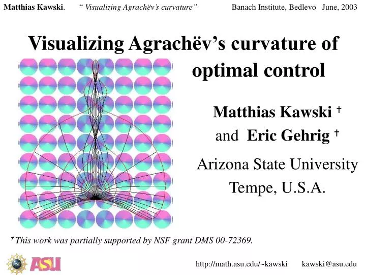
Visualizing Agrachëv’s curvature of optimal control Matthias Kawski and Eric Gehrig Arizona State University Tempe, U.S.A. This work was partially supported by NSF grant DMS 00-72369. http://math.asu.edu/~kawskikawski@asu.edu
Outline • Motivation of this work • Brief review of some of Agrachëv’s theory, and of last year’s work by Ulysse Serres • Some comments on ComputerAlgebraSystems “ideally suited” “practically impossible” • Current efforts to “see” curvature of optimal cntrl. • how to read our pictures • what one may be able to see in our pictures • Conclusion: A useful approach? Promising 4 what? http://math.asu.edu/~kawskikawski@asu.edu
Purpose/use of curvature in opt.cntrl Maximum principle provides comparatively straightforward necessary conditions for optimality,sufficient conditions are in general harder to come by, and often comparatively harder to apply.Curvature (w/ corresponding comparison theorem)suggest an elegant geometric alternative to obtain verifiable sufficient conditions for optimality compare classical Riemannian geometry http://math.asu.edu/~kawskikawski@asu.edu
Curvature of optimal control • understand the geometry • develop intuition in basic examples • apply to obtain new optimality results http://math.asu.edu/~kawskikawski@asu.edu
Classical geometry: Focusing geodesics Positive curvature focuses geodesics, negative curvature “spreads them out”. Thm.: curvature negative geodesics (extremals) are optimal (minimizers) The imbedded surfaces view, and the color-coded intrinsic curvature view http://math.asu.edu/~kawskikawski@asu.edu
Definition versus formula A most simple geometric definition - beautiful and elegant. but the formula in coordinates is incomprehensible (compare classical curvature…) (formula from Ulysse Serres, 2001) http://math.asu.edu/~kawskikawski@asu.edu
Aside: other interests / plans • What is theoretically /practically feasible to compute w/ reasonable resources? (e.g. CAS: “simplify”, old: “controllability is NP-hard”, MK 1991) • Interactive visualization in only your browser… • “CAS-light” inside JAVA (e.g. set up geodesic eqns) • “real-time” computation of geodesic spheres (e.g. “drag” initial point w/ mouse, or continuously vary parameters…) “bait”, “hook”, like Mandelbrot fractals…. Riemannian, circular parabloid http://math.asu.edu/~kawskikawski@asu.edu
References • Andrei Agrachev: “On the curvature of control systems” (abstract, SISSA 2000) • Andrei Agrachev and Yu. Sachkov: “Lectures on Geometric Control Theory”, 2001, SISSA. • Ulysse Serres: “On the curvature of two-dimensional control problems and Zermelo’s navigation problem”. (Ph.D. thesis at SISSA) ONGOING WORK ??? http://math.asu.edu/~kawskikawski@asu.edu
From: Agrachev / Sachkov: “Lectures on Geometric Control Theory”, 2001 http://math.asu.edu/~kawskikawski@asu.edu
From: Agrachev / Sachkov: “Lectures on Geometric Control Theory”, 2001 http://math.asu.edu/~kawskikawski@asu.edu
From: Agrachev / Sachkov: “Lectures on Geometric Control Theory”, 2001 Next: Define distinguished parameterization of H x http://math.asu.edu/~kawskikawski@asu.edu
The canonical vertical field v http://math.asu.edu/~kawskikawski@asu.edu
From: Agrachev / Sachkov: “Lectures on Geometric Control Theory”, 2001 http://math.asu.edu/~kawskikawski@asu.edu
Jacobi equation in moving frame Frame or: http://math.asu.edu/~kawskikawski@asu.edu
Zermelo’s navigation problem “Zermelo’s navigation formula” http://math.asu.edu/~kawskikawski@asu.edu
formula for curvature ? total of 782 (279) terms in num, 23 (7) in denom. MAPLE can’t factor… http://math.asu.edu/~kawskikawski@asu.edu
Use U. Serre’s form of formula polynomial in f and first 2 derivatives, trig polynomial in q, interplay of 4 harmonics so far have still been unable to coax MAPLE into obtaining this without doing all “simplification” steps manually http://math.asu.edu/~kawskikawski@asu.edu
First pictures: fields of polar plots • On the left: the drift-vector field (“wind”) • On the right: field of polar plots of k(x1,x2,f)in Zermelo’s problem u* = f. (polar coord on fibre)polar plots normalized and color enhanced: unit circle zero curvature negative curvature inside greenish positive curvature outside pinkish http://math.asu.edu/~kawskikawski@asu.edu
Example: F(x,y) = [sech(x),0] k NOT globally scaled. colors for k+ and k- scaled independently. http://math.asu.edu/~kawskikawski@asu.edu
Example: F(x,y) = [0, sech(x)] Question: What do optimal paths look like? Conjugate points? k NOT globally scaled. colors for k+ and k- scaled independently. http://math.asu.edu/~kawskikawski@asu.edu
Example: F(x,y) = [ - tanh(x), 0] k NOT globally scaled. colors for k+ and k- scaled independently. http://math.asu.edu/~kawskikawski@asu.edu
From now on: color code only(i.e., omit radial plots) http://math.asu.edu/~kawskikawski@asu.edu
Special case: linear drift • linear drift F(x)=Ax, i.e., (dx/dt)=Ax+eiu • Curvature is independent of the base point x, study dependence on parameters of the driftkA(x1,x2,f) = k(f,A)This case is being studied in detail by U.Serres.Here we only give a small taste of the richness of even this very special simple class of systems http://math.asu.edu/~kawskikawski@asu.edu
Linear drift, preparation I • (as expected), curvature commutes with rotationsquick CAS check: > k['B']:=combine(simplify(zerm(Bxy,x,y,theta),trig)); http://math.asu.edu/~kawskikawski@asu.edu
Linear drift, preparation II • (as expected), curvature scales with eigenvalues(homogeneous of deg 2 in space of eigenvalues)quick CAS check: > kdiag:=zerm(lambda*x,mu*y,x,y,theta); Note: q is even and also depends only on even harmonics of q http://math.asu.edu/~kawskikawski@asu.edu
Linear drift • if drift linear and ortho-gonally diagonalizable then no conjugate pts(see U. Serres’ for proof, here suggestive picture only) > kdiag:=zerm(x,lambda*y,x,y,theta); http://math.asu.edu/~kawskikawski@asu.edu
Linear drift • if linear drift has non-trivial Jordan block then a little bit ofpositive curvature exists • Q: enough pos curv forexistence of conjugate pts? > kjord:=zerm(lambda*x+y,lambda*y,x,y,theta); http://math.asu.edu/~kawskikawski@asu.edu
Some linear drifts Question: Which case is good for optimal control? diag w/ l=10,-1 diag w/ l=1+i,1-i jordan w/ l=13/12 http://math.asu.edu/~kawskikawski@asu.edu
Ex: A=[1 1; 0 1]. very little pos curv http://math.asu.edu/~kawskikawski@asu.edu
Scalings: + / - , local / global same scale for pos.& neg. parts global color-scale, same for every fibre here: F(x) = ( 0, sech(3*x1)) local color-scales, each fibre independ. pos.& neg. parts color-scaled independently http://math.asu.edu/~kawskikawski@asu.edu
Example:F(x)=[0,sech(3x)] scaled locally / globally http://math.asu.edu/~kawskikawski@asu.edu
F(x)=[0,sech(3x)] • globally scaled. • colors for k+ and k- scaled simultaneously. http://math.asu.edu/~kawskikawski@asu.edu
F(x)=[0,sech(3x)] • globally scaled. • colors for k+ and k- scaled simultaneously. http://math.asu.edu/~kawskikawski@asu.edu
Conclusion • Curvature of control: beautiful subject promising to yield new sufficiency results • Even most simple classes of systems far from understood • CAS and interactive visualization promise to be useful tools to scan entire classes of systems for interesting, “proof-worthy” properties. • Some CAS open problems (“simplify”). Numerically fast implementation for JAVA???? • Zermelo’s problem particularly nice because everyone has intuitive understanding, wants to argue which way is best, then see and compare to the true optimal trajectories. http://math.asu.edu/~kawskikawski@asu.edu