Download

1 / 34
340 likes | 524 Views
Normal Mapping for Precomputed Radiance Transfer. Peter-Pike Sloan Microsoft. Inspiration. [McTaggart04] Half-Life 2 “Radiosity Normal Mapping”. Related Work. [Willmott99] Vector irradiance formulation of radiosity (for accelerating computation)

E N D
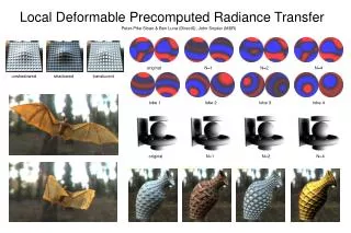
Normal Mapping for Precomputed Radiance Transfer Peter-Pike Sloan Microsoft
Inspiration • [McTaggart04] Half-Life 2 “Radiosity Normal Mapping”
Related Work • [Willmott99] Vector irradiance formulation of radiosity (for accelerating computation) • [Tabellion04] Lighting model similar to above (dominant light direction) • [Good2005] “Spherical Harmonic Light Maps”
Goal • Develop lightweight techniques to decouple normal variation (ala HL2) • From parameterized models of lighting (PRT) • For rigid objects • Non goals • Modeling “local GI” of the bumps [Sig05] • Masking effects • Glossy materials
Bi-Scale Radiance Transfer • l : vector = source radiance spherical function • Mp : 25x25 transfer matrix at point p (source → transferred incident) • q(xp) : ID map(2D → 2D, maps RTT patch over surface) • b(x,v): RTT (4D → 25D, tabulated over small spatial patch) applies macro-scale transferred radiance to meso-scale RTT
Bi-Scale Radiance Transfer • l : vector = source radiance spherical function • Mp : 25x25 transfer matrix at point p (source → transferred incident) • q(xp) : ID map(2D → 2D, maps RTT patch over surface) • b(x,v): RTT (4D → 25D, tabulated over small spatial patch) applies macro-scale transferred radiance to meso-scale RTT
Bi-Scale Radiance Transfer • l : vector = source radiance spherical function • Mp : 25x25 transfer matrix at point p (source → transferred incident) • q(xp) : ID map(2D → 2D, maps RTT patch over surface) • b(x,v): RTT (4D → 25D, tabulated over small spatial patch) applies macro-scale transferred radiance to meso-scale RTT
Limitations • Expensive • Stores 64 “response vectors” that are 9-36D (x3 for spectral) • Parallax mapping cheaper way of getting masking • Local radiance is too much data (9 – 36 x 3) for low res textures/per-vertex • Add constraints • Just model normal variation • Diffuse only
Diffuse + Normal Maps • Quadratic SH [Ramamoorthi2001] Distant Lighting Environment
Diffuse + Normal Maps • Quadratic SH [Ramamoorthi2001] Distant Radiance to Transferred Incident Radiance In local frame
Diffuse + Normal Maps • Quadratic SH [Ramamoorthi2001] Diagonal Convolution Matrix Clamped cosine kernel
Diffuse + Normal Maps • Quadratic SH [Ramamoorthi2001] Irradiance Environment Map
Diffuse + Normal Maps • Quadratic SH [Ramamoorthi2001] Irradiance Environment Map
Diffuse + Normal Maps • Quadratic SH [Ramamoorthi2001] Evaluate SH basis with normal
Concerns • Lot of data at low res • 9xO2 matrices (x3 with color bleeding) • Can compress using CPCA [Sig03] • Too much data passed from low res to high res • Irradiance emap (27 numbers, 7 interpolators) • Alternatives • Project into analytic basis • Separable approximation
Analytic Basis Project into new basis (fewer rows)
Shifted Associated Legendre Polynomials [Gautron2005]
Comparison PRT Gold Standard HL2 SAL
Comparison PRT Gold Standard HL2 SAL
Normal Mapping for PRT • Use same ideas as BRDF factorization [Kautz and McCool1999] Bi-linear basis functions over hemisphere (4 non-zero) Matrix, rows “normal directions” columns quadratic SH light Aij equals evaluating convolved light basis function “j” in normal direction “i”
Normal Mapping for PRT • Compute SVD of A Nx9 matrix (each column is a “normal basis” texture) 9x9 diagonal matrix (singular values) 9x9 matrix
Normal Mapping for PRT • Old equation • New equation
Normal Mapping for PRT • Use first M singular values • MxO2 matrix • M channel “normal direction” texture
Pixel Shader StandardSVDPS( VS_OUT In, out float3 rgb : COLOR ) { float2 Normal = tex2D(NormalSampler, In.TexCoord); float2 vTex = Normal*0.5 + float2(0.5,0.5); float4 vU = tex2D(USampler,vTex); rgb.r = dot(In.cR,vU); rgb.g = dot(In.cG,vU); rgb.b = dot(In.cB,vU); rgb *= tex2D(AlbedoSampler, In.TexCoord); }
Conclusions • Lightweight form of normal mapping for PRT • Inspired by Half-Life 2 • For static objects, diffuse only • HL2 basis and separable basis seem to be best • Experiment with CPCA more [Sig03] • Integrate with other techniques • Parallax mapping for masking • Ambient Occlusion for local effects
Acknowledgments • Gary McTaggart for HL2 images • Shanon Drone for Models • Paul Debevec for Light Probes