Download
1 / 36
360 likes | 493 Views
Clustered Principal Components for Precomputed Radiance Transfer. Peter-Pike Sloan Microsoft Corporation Jesse Hall, John Hart UIUC John Snyder Microsoft Research. Demo. PRT Terminology. PRT Terminology. PRT Terminology. PRT Terminology. PRT as a Linear Operator.

E N D
Clustered Principal Components for Precomputed Radiance Transfer Peter-Pike Sloan Microsoft Corporation Jesse Hall, John Hart UIUC John Snyder Microsoft Research
PRT as a Linear Operator • l : light vector (in source basis) • Mp : source-to-exit transfer matrix • ep: exit radiance vector (in exit basis) • y(vp) : exit basis evaluated in direction vp • ep(vp) : exit radiance in direction vp
PRT Special Case: Diffuse Objects transfer vector rather than matrix [PRT02] SH [Xi03] Directional [Ng03] Haar [Ashikhmin02] Steerable • independent of view (constant exit basis) • matrix is row vector • previous work uses different light bases • image relighting
PRT Special Case: Surface Light Fields transfer vector rather than matrix [Miller98] [Nishino99] [Wood00] [Chen02] [Matusik02] • frozen lighting environment • matrix is column vector
Factoring PRT (BRDFs) • Tp: source → transferred incident radiance • Rp : rotate to local frame • B: integrate against BRDF [Westin92] • y(vp) •ep: evaluate exit radiance at vp
Hemispherical Projection • exit radiance is defined over hemisphere, not sphere • spherical harmonics not orthogonal over hemisphere • how to project hemispherical functions using SH? • naïve projection assumes “underside” is zero • least squares projection minimizes approximation error • see appendix
Extending PRT to BSSRDFs • already handled by original equation • use [Jensen02], only multiple scattering (matrix with only 1 row) • mix with “conventional” BRDF
Problems With PRT • Big matrices at each surface point • 25-vectors for diffuse, x3 for spectral • 25x25-matrices for glossy • at ~50,000 vertices • Slows glossy rendering (4hz) • Frozen View/Light can increase performance • Not as GPU friendly • Limits diffuse lighting order • Only very soft shadows
Compression Goals • Decode efficiently • As much on the GPU as possible • Render compressed representation directly • Increase rendering performance • Make non-diffuse case practical • Reduce memory consumption • Not just on disk
Compression Example Surface is curve, signal is normal
Compression Example Signal Space
VQ Cluster normals
VQ Replace samples with cluster mean
PCA Replace samples with mean + linear combination
CPCA Compute a linear subspace in each cluster
CPCA • Clusters with low dimensional affine models • How should clustering be done? • Static PCA • VQ, followed by one-time per-cluster PCA • optimizes for piecewise-constant reconstruction • Iterative PCA • PCA in the inner loop, slower to compute • optimizes for piecewise-affine reconstruction
Related Work • VQ+PCA [Kambhatla94] (static) • VQPCA [Khambhatla97] (iterative) • Mixture PC [Dony95] (iterative) • More sophisticated models exist • [Brand03], [Roweis02] • Mapping to current GPUs is challenging • Variable storage per vertex • Partitioning is more difficult (or requires more passes)
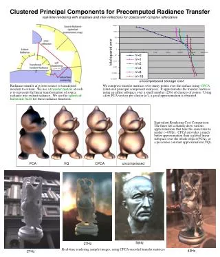
Equal Rendering Cost VQ PCA CPCA
Rendering with CPCA Constant per cluster – precompute on the CPU Rendering is a dot product Compute linear combination of vectors Only depends on # rows of M
Non-Local Viewer • Assume: • vp constant across object (distant viewer) Rendering independent of view & light orders - linear combination of colors
+ = + Rendering
2 2 1 3 2 2 2 2 2 2 2 2 1 3 2 2 2 1 Overdraw • faces belong to 1-3 clusters • OD = 1 face drawn once • OD = 2 face drawn 2x • OD = 3 face drawn 3x • coherence optimization: • reclassification • superclustering
Texture Constants Exit Rad. GPU Dataflow Vertices Vertex Shader PixelShader
Results All examples have 25x25 matrices, 256 clusters, 8 PCA vectors
Conclusions CPCA • works in “signal space”, not “surface space” • uses affine subspace per-cluster • compresses PRT well • is used directly without “blowing out” signal • requires small, uniform state storage • provides • faster rendering • higher-frequency lighting
Future Work • time-dependent and parameterized geometry • higher-frequency lighting • combination with bi-scale rendering • better signal continuity
Questions? • DirectX SDK for PRT available soon. • Jason Mitchell, Hugues Hoppe, Jason Sandlin, David Kirk • Stanford, MPI for models