Download
1 / 12
130 likes | 311 Views
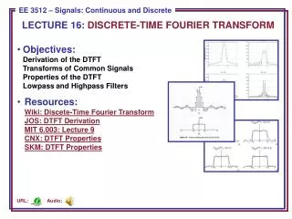
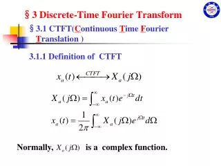
Chapter 4 Fourier Transform of Discrete-Time Signals 2 nd lecture Mon. June 17, 2013. 4.1 Discrete-Time Fourier Transform. Continuous-time F.T . from Chapt . 3:. CTFT. Now, the input is x[n]. Define Discrete-time F.T .:. DTFT. Inverse DTFT (4.1.3, p. 175). Eq. 4.27:.

E N D
Chapter 4Fourier Transform of Discrete-Time Signals2nd lectureMon. June 17, 2013
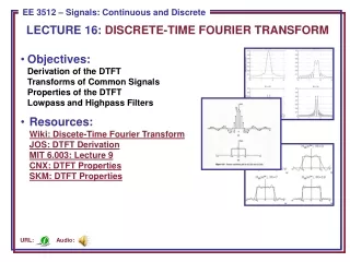
4.1 Discrete-Time Fourier Transform • Continuous-time F.T. from Chapt. 3: CTFT • Now, the input is x[n]. Define Discrete-time F.T.: DTFT
Inverse DTFT (4.1.3, p. 175) • Eq. 4.27:
Example 4.3 – Rectangular Pulse, cont’d Even signal, so DTFT is purely real. Use the def. (Eq. 4.2) and follow Ex. 4.1 to get:
Example 4.3 – Rectangular Pulse, cont’d MATLAB code* to plot magnitude: *This script can be found on the class website with the filename dtft_pulse.m
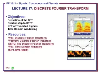
Sect. 4.2 – Discrete Fourier Transform (DFT / FFT) This is arguably the most important result in all of signal processing and modern communication.
Frequency Domain Voltage “Hello” Frequency
Discrete Fourier Transform Need to store the transform in computer memory & files. DFT: Inverse DFT:
Discrete Fourier Transform N-point DFT is computed using the FFT algorithm. DFT: MATLAB: n=1:1024; x=(-.7).^n; xf=fft(x); stem(xf)
Discrete Fourier Transform N-point DFT: N is always 2n in practice. Common values are 1024, 4096. First point is k = 0, last point is k = N-1, center point is N/2. Magnitude is symmetric around N/2: |X(N-1)|=|X(1)|, |X(N-2)|=|x(2)|, …