Download
1 / 55
550 likes | 647 Views
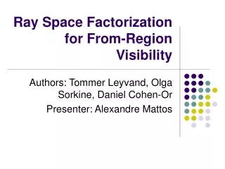
Ray Space Factorization for From-Region Visibility. Tommer Leyvand Olga Sorkine Daniel Cohen-Or Tel-Aviv University, Israel. From-Region Visibility. Problem of identifying which parts are visible from a region (viewcell). Visibility Set Valid from within the viewcell. Entire Model.

E N D
Ray Space Factorization for From-Region Visibility Tommer Leyvand Olga Sorkine Daniel Cohen-Or Tel-Aviv University, Israel
From-Region Visibility Problem of identifying which parts are visible from a region (viewcell) Visibility Set Valid from within the viewcell Entire Model
Abstract • Conservative occlusion culling method • Factorizing 4D visibility problem in to horizontal and vertical components • Two components is solved asymmetrically • Horizontal component • Parameterization of the ray space • Vertical component • Incrementally merging umbrae
Abstract • Efficiently realized together by modern graphics hardware • Occlusion map to encode visibility • Culling time and size of the computed PVS→ depend on the size of the viewcell • For moderate viewcells • Occlusion culling of large urban scenes:< 1 sec • Size of the PVS = 2 * size of the exact VS
Dimensionality ofFrom-Region Visibility From-Region visibility is 4D • A ray exists the viewcell through a 2D surface and enters the target region through a 2D surface viewcell
Our Factorization Factor the 4D visibility problem into horizontal and vertical components Ray Space Approach Umbra Merging Approach Horizontal direction Vertical direction
Form-Pint vs. From-Region • Complexity of models keeps growing • Occlusion culling can effectively reduce the rendering depth complexity • Visibility from-point: compute each frame • Visibility from-region: valid for a region rather than a single point • Advantage of time and spatial coherence • Computational cost is amortized over consecutive frames • Compute from-region visibility on-the-fly,not having to resort to off-line methods
4-Dimensional Problem • Decide: whether an object S is (partially) visible or occluded from a region C • Requires detecting:whether there exists at least a single ray thatleaves C and intersects Sbefore it intersects an occluder ? C S region occluder object
Solutions • Exact solutions are possible:[Nirenstein et al. 2002…]!overly expensive! • Conservative solutions: [Durand et al. 2000…]gain speed-up by overestimating the exact VS • Dealing with 2.5D scenes: [Koltun et al. 2001…]2.5D occluders is quite reasonable in practice(especially in walkthrough applications) • For more general scenes • Necessary to have a culling method thatcan deal withthe occlusion of a larger domain of shapes
Graphics Hardware • Advanced graphics cards: visibility featureindicates whether a just drawn polygon is visible or hidden by polygons already drawn • The technique this paper present here:utilizes capabilities of the latest graphics hardware to accelerate the performance for from-region visibility
Occlusion Culling Method • Occlusion cast: arbitrary 3D models • Idea: 4D visibility problem → two 2D components • Horizontal: parameterization of the ray space • Vertical: maintained by pairs of occluding angles • Key point: • Horizontal components → polygonal shapes • Each point in polygonal footprints → vertical slice • Modern graphics hardware → polygonal footprints can be drawn • Applying per-pixel visibility calculations →significant speed-up
From-region Method • Early generic from-region methods:occlusion of a single occluder or approximated • Better capture the occlusion and reduce the VS: detect objects – hidden by a group of occluders • Advanced from-region methods:aggregating individual umbrae into a large umbra capable of occluding larger parts of the scene
Aggregating Umbrae • Ray-parameterization: • capture the visibility of an object into some geometric region (a polygonal footprint) • Apply Boolean operations (visibility) • Fuses individual intersecting umbrae into large umbrae • Combines these two approaches!
Occlusion Problem • Visibility problems: (in particular occlusion problem) → problems in line spaces • Example: basic occlusion problemGiven a segment C, an object A is occluded from any point on C by a set of objects Bi →if all the lines intersecting C and Aalso intersect the union of Bi A C
Occlusion Problem – Solution • Using the line space,lines in the primal space mapped to points • Mapping: 2D line vs. pointDefine: By coefficients of the lines (primal space) line y = ax + bis mapped topoint (a, -b) (in the line parameter space) footprint A C
Occlusion Problem – Analysis • Not optimal: vertical lines are mapped to infinity • Problem: all lines with large coefficients • Practical reason: dual space must be bounded • Solution: moving to higher dimensions • Loses the simplicity and efficiencyof operating in image space
Occlusion Problem – Analysis • Ideas to 3D case: not as easy as in 2Dthe parameter space of 3D lines has high D • In general, 3D lines have four DOF • Rays: origin of the lines • Visibility in 2D flatland: limited interest • Note: most of objects are detected as occluded in flatland, while actually being visible in 2.5D due to their various heights
Occluder Fusion • Different approach for occluder fusion:incrementally construct an aggregate umbra in primal space • Occluder fusion occurs whenever:individual umbrae intersect • Note: umbra intersection is a sufficient condition but not necessary one
Overview • Bounded nonsingular parameterization:2D component by a vertical projection of the objects onto the ground (z=0) • Footprint:composed of a polygons (parameter space) • Rays in 3D primal space = (s,t) direction define a vertical slice (directional plane)
Overview Line segment: casts a directional umbra→ each directional plane: aggregated umbra (occluder)→ aggregated umbra (all): maintained in occlusion map
Overview • Hierarchical front to back traversal of objects • Perform visibility queries • Update the occlusion map • Footprint of objects • Conservatively discretized • Drawn by the graphics hardware • Occlusion map • Represented by a discrete ray space
Ray Parameterization • Duality of R2is a correspondence between • 2D linesy=ax+bin the primal space • Points (a,-b) in the dual space • Different parameterization of 2D lines • Only the oriented lines (rays) (emerge from a given 2D square viewcell) • Not have singularity • Parameter space is bounded • Rays (leave the viewcell) intersect a triangle • Form a footprint in the parameter space • Can be represented by a few polygons
t=0 1/4 s=0 1/4 3/4 1/2 3/4 1/2 Primal Space • s, t: associated with theinner, outer squares • r(sr, tr) : ray r intersects with inner and outer squares Primal Space
t=0 1/4 s=0 1/4 3/4 1/2 3/4 1/2 Footprint of a 2D Triangle • Footprint: a geometric primitiveas the set of all points in the parameter spacethat refer to rays that intersect the primitive t 1/2 tq1(1/4) q1 tq1(1) tq1(1/2) tq1(3/4) tq1(1/4) A tq1(1/2) q2 1/4 s 0 1/2 3/4 1 1/4 Primal Space Ray Parameter Space -- For a fixed value of s: { (s,t) : t [tq1(s), tq2(s)] }
t=0 1/4 s=0 1/4 3/4 1/2 3/4 1/2 Footprint of a 2D Triangle t=1/4 t=1/2 s=1/4 s=1/2
Visibility within a Vertical Plane • Traverse the cells of a kd-tree in a front-to-back order interleave occlusion tests against the occlusion map andumbra merging to maintain it • How to perform visibility queries? • How to perform occluder fusion?
Vertical Slice The visibility is solved within each vertical slice A vertical slice Within a vertical slice Vertical direction Horizontal direction
Vertical slice R R ‘ t s Horizontal direction Vertical Visibility Query • B cast a directional umbrawith respect to K within P(s,t) • Supporting-angles encode the directional umbra of B within the vertical plane P(s,t) • Angle values are represented by their tangentsas functions of (s,t) P(s,t) : vertical planeB = p1p2 , : supporting line , : supporting angle p1 B p2 K
Vertical Visibility Query • Q: line segment within P(s,t) that’s behind B(according to the front-to-back order with respect to the viewcell) • Determining whether Q is occluded by B→Testing whether the umbra of B contains Q • Front-to-back order guarantees • tested segment is always behind the occluders→supporting lines are sufficient for the visibility test Directional accumulated umbra Q is occluded: Both of their endpoints are within the accumulated umbrai.e. Within a slice: Test occlusion by comparing supporting angles
Merging Umbrae • In the vertical direction plane • umbra aggregation is performed by testing umbra intersection and fusing occluders • Supporting lines alone do not uniquely describe the umbra Adding separating lines→ defining the umbra uniquely
Merging Umbrae (1) Umbra of one segment is contained in the area between the supporting lines of the other segment “throw out” the contained segment and keep just the other one
Merging Umbrae (2) No umbra intersection occurs
Merging Umbrae (3) If (1)(2) tests fail as well → umbra intersection Replace the two segments by a new “virtual” occluder segment Insert into the occlusion map the following angles:
Occluder Fusion • Note: • Fused umbra is valid only for testing occlusion of ocludees placed behind all the occluders that created the umbra • Merging umbra is order-independent • an approximate ordering of the occluders is more efficient • Typically man-made scenes have a strong vertical coherence andafter some umbra-merging steps, the umbra grows to capture most of the occlusion
Putting It All Together • Combine: horizontal footprint, vertical visibility • Exploiting-all the directional (vertical) computations can be performed in parallel • Footprints are conservatively discretized before rendering • adding four values {v0,v1,v2,v3} to each pixels • represent the four supporting and separating angles
v t (s,t) s Parameter Space Umbra Encoding • For each vi: • footprint F(R’) is augmented into a 3D (s,t,v) parameter space, yielding four 3D footprints • these footprints are surface Vertical direction Horizontal direction
Hierarchical VisibilityCulling • Original objects of the scene are inserted into a kd-tree • During the algorithm, kd-tree has two functions • traverse the scene in a front-to-back order • allows culling of large portions of model
Kd-tree traverse • Kd-tree is traverse top-down • large cells can be detected as hidden and culled with all their sub-tree • if a leaf node is still visible • the visibility of each bounding box associated with it is tested • if a bounding box is visible • the triangles bounded in it are defined as potentially visible
Occlusion • In scenes with significant occlusion • objects close to the viewcell rapidly fill the occlusion map • most of the back larger kd-cells are detected as hidden • From-region front-to-back order of the kd-cells is a strict order rather than approximate • guaranteed by using large kd-cells whose splitting planes never intersect any viewcells
Merging Umbra • Merging umbra is applied while traversing the kd-tree front-to-back • a leaf node is detected as visible • the polygons in that leaf are considered as occludersand their footprint are inserted into the occlusion map(possibly merging with the existing umbrae created so far) • Merging umbraesimplifies the occlusion map and increases the occlusion • optionally, before updating the occlusion map, the visibility of individual polygons in the PV leaf can be tested to tighten the PVS
Algorithm PVS← CalculateVisibility(kd-tree.root) CalculateVisibility(curr_kd_cell) if TestVisibility(curr_kd_cell) //current kd-cell is visible if cur_kd_cell.IsLeaf() PVS←PVS curr_kd_cell.getTriangles() AugmentOcclusionMap(curr_kd_cell.getRriangles()) else foreach kd_child curr_kd_cell.children in f2b order CalculateVisibility(kd_child) end foreach endif else return//current kd-cell occluded->terminate end
2.5D Occluders • 2.5D occluders: “half-umbra” • only top supporting angle is stored • bottom supporting angle is always zero • encode using the z-coordinate of the 2D footprint • Testing visibility of an occludee • testing the visibility of its footprint (disabling z-buffer) • Umbra fusion by • enabling z-buffer updates • drawing the occluder footprint
3D Occluders • Use a series of top and bottom supporting and separating angles • Occlusion map stores only a single directional umbra per direction (hardware limitation) • Testing visibility of an occludee • testing whether the top or bottom supporting footprints are visible • Umbra fusion by • testing whether the new umbra intersects the current umbra in the occlusion map
Implementation • Cg implementation: • 32bit floating-point PBuffer • store the global occlusion map • Fragment shader functionality • calculation of the directional umbra within each slice • testing occlusion • merging umbra
Urban Model • 2GHz P4 machine with Nvidia GeForce4 Ti graphics card • A randomly generated urban model: • Large set of parameters • Increasing vertical complexity • Not axis-aligned
Non-realistic Model • Box-field: consists of randomly generated boxes • Not too dense → geometry deep inside the box-field is visible • Reducing the effectiveness of the use of a hierarchy
Result-Urban Scene • 26.8M triangles • Height of viewcells: 2.5 units • PVS and VS size is given in triangles • Time: refers to culling-time (seconds) • Off-junction viewcells: within some city block • In-junction viewcells: on the junction of two long avenues
Result- Box-field • 20.7M triangles • Height of viewcells: 10 units • Near viewcell: viewcell located from within the field • Far viewcell: viewcell located outside and far from the field • When the viewcell is closer to the scene,the objects are larger and occlude much more
Result-Culling effectiveness • Comparison between: 2.5D vs. 3D occluders • 20M triangles (urban city model) • Maintaining a single full umbrareducesthe size of the PVS,at the expense of longer computation time
Result • Culling time is directly dependent on two interdependent factors • number of visibility queries • number of visible triangles (occluders) • The technique can deal with a huge model • due to the hierarchy • but only as long as the size of the VS is small • only a small number of triangles is visible • implies that only a small number of kd-cells in the hierarchy is tested