Download
1 / 34
340 likes | 344 Views
This presentation discusses the need for defining natural background visibility in the VISTAS region and provides insights into current scientific knowledge. It also explores options and next steps for estimating natural background visibility.

E N D
Options for Estimating Natural Background Visibility in the VISTAS Region Ivar Tombach with benefit of material prepared by Jim Boylan and Daniel Jacob (Harvard University) Presentation to VISTAS Workgroups 15 January 2004
The Need • VISTAS needs to define natural background visibility in 2064 and required rate of progress by 2018 • due Summer 2004 • Definitions should be specific for each VISTAS Class I area
Presentation Objective • Identify issues related to estimating natural background visibility • Provide insights into current scientific knowledge • Discuss options and next steps (Update of 9/24/03 presentation by Jim Boylan)
VISTAS Questions • Should we use the EPA default values to determine natural extinction at Class I Areas in the VISTAS states? • How can the EPA default values be refined and adjusted to better reflect local conditions? • How do we deal with the impact of intercontinental transport of anthropogenic emissions on natural background conditions? • What are the policy implications of adjusting the EPA’s recommended approach?
EPA’s Default Natural Conditions for the East 1Trijonis, et al, 1990. National Acid Precipitation Assessment Program, State of Science Report #24.
EPA’s Approach for Determining Natural Extinction on 20% Haziest Days at a Class I Area • Start with default values • Increase sulfate and nitrate extinction for particle growth due to humidity, using climatological-average f(RH) for site • Add 10 Mm-1 for Rayleigh (clear air) scattering • Use Ames & Malm statistical procedure to determine 90th percentile value It’s all in EPA’s guidance document.
Key Formulas Light Extinction (Mm-1) • bext = 3*f(RH)*[SO4] + 3*f(RH)*[NO3] + 4*[ORG] + 10*[EC] + 1*[Soils] + 0.6*[PMC] + bRay • bRay= 10 Mm-1 Haze Index (dv) • HI = 10 ln (bext/bRay)
Example: Great Smoky Mountains(Annual Average Default Natural Background)
Major Issues with Default Approach • Default Concentrations • Same concentrations assumed at all Class I areas in the East • Same concentrations assumed to occur every month of the year • Fine sea salt and associated water not included • Calculation of 20% Haziest Days • Same frequency distribution assumed for every Class I area in the East In other words, the approach assumes one size fits all.
More Major Issues • In Calculation of 20% Haziest Days • 90th %-ile assumed to represent haziest 20% • Organics not rolled back when estimating standard deviation
Possible Refinements to Default Approach for VISTAS • Fix Ames and Malm statistical procedure to reflect 20% haziest days -- adds 0.42 dv • Lowenthal and Kumar, 2003 • Change carbon mass multiplier from 1.4 (urban) to 2.1 (rural) to better represent natural conditions • Turpin and Lim, 2001 • OC is the biggest contributor to default natural extinction, so this substantially affects the assumed natural background
Possible Refinements (cont’d) • Consider oceanic aerosol impacts (sea salt and organics) near coast • Average fine sea salt concentration estimates range from 0.3 to 1.3 µg/m3 at Cape Romain and Florida IMPROVE sites • Salt is hygroscopic, so extinction impact is greater than for same amount of (non-hygroscopic) soil, although size distributions are similar • Oceanic organic particle concentration ~0.3 µg/m3 • Review default soil concentrations • Current concentrations approximate default in northern portion of VISTAS region ==> Default may be too large there
Possible Refinements (cont’d) • Consider biogenic organic carbon (and, perhaps, sulfur) from forests • Fine OC ~ 9 µg/m3 during growing season in tropics • Emission flux in some SE forests in summer could be comparable to that in tropics, although annual average emissions flux is less • Consider carbon (EC and OC) impacts from natural fires • Global modeling suggests mean naturally-emitted EC and OC in the East approximate the default concentrations
Possible Refinements (cont’d) • Consider episodic impact of intercontinental dust transport • Episodic African dust impacts are frequently greater than 3 µg/m3 in June-August in southern part of VISTAS region • Episodic Asian dust impacts are greater than 1 µg/m3 from spring through fall in northern part of VISTAS region • These episodic concentrations exceed the average soil default value of 0.5 µg/m3 • Consider impact of intercontinental sulfate and nitrate transport (mostly anthropogenic) • Global modeling suggests mean transported sulfate and nitrate concentrations are ~2-3 times the default concentrations
The $64,000 Question • How much of each of these possible refinements is already reflected in the default values? • Clearly -- • Default organics multiplier and Ames & Malm statistical factor should be changed • Some VISTAS locations clearly differ substantially from the default averages for entire East, at least during part of the year • Coastal salt and organics • African dust in summer • Forest organics during growing season • Episodic carbon from natural fires
Potential Impacts of Some Refinements on Dry Extinction in VISTAS Region Blue = International Anthropogenic Transport Adjustment ; Red = Natural BackgroundRefinement ** This value represents a hypothetical worst case scenario including episodic effects (e.g., Everglades in the summertime)
Potentially Biggest Effects • All year • Ames & Malm statistics • OC multiplier factor • Sea salt in coastal areas • Oceanic carbon in coastal areas • Part time • Forest organics during growing season • African dust in summer in the south, especially during episodes • Asian dust during episodes in the north, spring to fall • OC and EC from wildfires, episodic
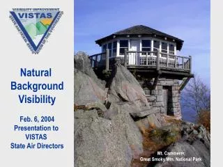
Implications for VISTAS(Example: Great Smoky Mountains) • (1) Default situation: • Current extinction over 20% haziest days = 203 Mm-1 (30.1 dv) • Default 2064 natural conditions goal = 31.4 Mm-1 (11.44 dv) • Needed improvement over 60 years = 18.7 dv, or 3.11 dv per decade • Requires reduction of non-Rayleigh extinction by 28% per decade
GRSM Implications (cont’d) • (2) Example with refined natural conditions • Increase natural extinction on 20% haziest days in 2064 by 4 Mm-1 (especially, change organics multiplier and add some forest organics), • This decreases the required slope to 2.9 dv per decade, corresponding to a reduction in non-Rayleigh extinction by 26% per decade
GRSM Implications (cont’d) • (3) Most hazy days are in summer at GRSM • Add 7 Mm-1 for African dust and peak impacts of vegetation emissions • This further decreases the required slope to 2.5 dv per decade, corresponding to a reduction in non-Rayleigh extinction by 24% per decade
GRSM Implications (cont’d) If only sulfates are reduced, then neededSO2 reductions for the three scenarios are • (1) 54% per decade • (2) 38% per decade • (3) 30% per decade
Implications (cont’d)(Another Example: Cape Romain) • (1) Default situation: • Current extinction over 20% haziest days = 142 Mm-1 (26.5 dv) • Default 2064 natural conditions goal = 31.1 Mm-1 (11.36 dv) • Needed improvement over 60 years = 15.2 dv, or 2.53 dv per decade • Requires reduction of non-Rayleigh extinction by 24% per decade
ROMA Implications (cont’d) • (2) Example with refined natural conditions • Increase natural extinction on 20% haziest days in 2064 by 7 Mm-1 (same as GRSM plus sea salt and oceanic organics) • This decreases the required slope to a bit more than 2.1 dv per decade, corresponding to a reduction in non-Rayleigh extinction by 21% per decade
ROMA Implications (cont’d) • (3) If most hazy days are in summer at ROMA • Add 3 Mm-1 for African dust (no further vegetation adjustment here) • This further decreases the required slope to a bit leas than 2.1 dv per decade, corresponding to a reduction in non-Rayleigh extinction by 20% per decade
ROMA Implications (cont’d) If only sulfates are reduced, then needed SO2 reductions for the three scenarios are • (1) 32% per decade • (2) 28% per decade • (3) 27% per decade
Intercontinental Transport Issues • What do you do with the anthropogenicpollutants transported to the US from Mexico, Canada, and Asia? • Add their contributions to the natural background then determine the reasonable progress slope? • Don’t add them to the natural background, but account for them when you can not control anymore U.S. sources? • Can result in changing the slope of reasonable progress line • Similar implication as adding previously discussed refinements to EPA’s default extinction values
Intercontinental Transport (cont’d) 20% Haziest Days 29.9 dV Natural Background (with Intercontinental Transport) Natural Background 2000 YEAR 2064
Carbonaceous Aerosol from GEOS-CHEM Modeling *This includes anthropogenic vegetation burning, however. • Model indicates that EPA default natural concentrations are too low by factors of 2-3 except for OC and EC in Eastern U.S. – quantifying fire influences is critical • Transboundary pollution influences are relatively small compared to EPA default natural concentrations, except for EC from Canada/Mexico
Amm. sulfate (mg m-3) West East Amm. nitrate (mg m-3) West East Baseline (2001) 1.52 4.11 1.53 3.26 GEOS-CHEM- No anthro. emissions in US /globally • EPA default values 0.43/0.11 0.11 0.38/0.11 0.23 0.27/0.03 0.1 0.37/0.03 0.1 Contributions from trans-boundary anthro. sources Canada and Mexico Asia 0.15 0.13 0.14 0.12 0.20 -0.02 0.25 -0.02 Sulfate-Nitrate-Ammonium Aerosol from GEOS-CHEM Modeling • Achievability of EPA default estimates is compromised by transboundary pollution influences • Transboundary sulfate influence from Asia is comparable in magnitude to that from Canada + Mexico
Another Option…. • Couple the GEOS-CHEM global circulation model with the CMAQ regional air quality model • Annual simulation for 2002 • Time varying boundary conditions from GEOS-CHEM • Zero out U.S. anthropogenic emissions in CMAQ • Highly dependent on accurate inventory for biogenic and other natural emission sources • Provides site-specific natural background values
Caveat and Outlook • These results and conclusions are rough and tentative • They are based on limited review of literature • Our ability to provide site-specific, time varying estimates of natural levels should improve with further study of the literature • More relevant research results are being published regularly
Recommendations • Understand technical issues and policy implications (e.g., this conference call) • Interpret further data analyses by Air Resource Specialists (especially new coastal IMPROVE sites) • Decide on which default values to refine and approach for doing so • Cooperate with other RPOs on new natural background project (longer term)