Download
1 / 25
250 likes | 339 Views
Identifying Solar Wind Charge Exchange in XMM-Newton Observations. Jenny Carter & Steve Sembay University of Leicester. Aims of project. Identify XMM-Newton observations that have experienced SWCX enhancement during their exposure Identify key indicators of this effect

E N D
Identifying Solar Wind Charge Exchange in XMM-Newton Observations Jenny Carter & Steve Sembay University of Leicester
Aims of project • Identify XMM-Newton observations that have experienced SWCX enhancement during their exposure • Identify key indicators of this effect • Prepare test parameters • Apply to a set of archived observations • Analyse results with respect to test parameters • Look at application of test to whole archive and maybe create a tool for a user?
XMM-Newton and the Earth’s magnetosheath • 48 hour orbit • Pointing angle will sometimes pass through areas of high X-ray flux • Depends on pointing and time of year Earth Sun Robertson & Cravens 2003
Expected SWCX geocoronal X-ray flux characteristics • Emission lines (e.g. Snowden et al., 2004) • Short term variability • Local source, expect pointing dependence
Observations • XMM-Newton XSA archive • Control subjects • Kuntz & Snowden, 2008, A&A, 478, v2 • HDFN • Polaris Flare • Groth-Westfall strip • Snowden et al., 2004, HDFN • Around 200 observations (total currently ~1500 revs, ~4300 observations (MOS full-frame)) • Look at ACE data for each observation
Data preparation and tests Grade amount of scatter χ2 XSA Lightcurve testing ESAS filter data (EPIC MOS GOF) Remove sources Calculate variance each band ESAS create spectra “Ghost” sources Fin/Fout test Residual protons/flaring info (ESAS as well) XMM-Newton BGWG: http://xmm.vilspa.esa.es/external/xmm_sw_cal/background/index.shtml
ESAS and source removal • ESAS software: analysis of diffuse emission, filtering, diagnostic plots • Point source removal (2XMM catalogue) and ghosting Important for extra tests later on
Test • Test for variability in SWCX band i.e. OVIII (500 – 700 eV) • Compare to variability of continuum band (1100 – 1275 eV, 1600 – 1650 eV and 1900 – 2400 eV) • Test for a lack of correlation between the count rates • Test ok even for obs. with residual soft proton flaring • Other tests: check variance in each individual band compute in/out-FOV ratio (Fin_fout)
red-χ2; 3.635/10 red-χ2; 353.0/30
Results • Control observations with SWCX found in/out top set • ~11 observations with unpublished SWCX characteristics Ratio of variance in each band Large χ2 - SWCX obs. General trends:
ACE Example: obsn 0150680101 Oxygen and carbon ~Mp ~Bs Sun Earth
ACE Example: obsn 0149630301 MgXI?
ACE Example: obsn 0080515301 MgXI
Conclusions • Successful identification of control subjects • Identification of new cases of geocoronal SWCX emission (~11) • Some correlation with ACE • Some correlation with XMM-Newton pointing angle • Extreme case with many emission lines • Plans to extend diagnostic and grading technique to entire archive at Leicester
Plan • Geocoronal neutrals, SWCX and XMM-Newton • Search for correlation, choice of test • Observations used • Results – light curves • Results – spectra, redistributions of lines • Results – XMM-Newton position • Conclusion and future
ESAS filtering, basis • Main motivation for using ESAS: good for study of diffuse emission • Filtering based on GTIs to remove obvious soft proton contamination • Gives judge of residual soft proton contamination • Background spectra created from filter wheel closed data for particle-induced background
Previous method • Normalise lightcurves • Calculate difference between lightcurves • Calculate chi-squared distribution function • probability that a random variable will have a value greater than or equal to that for the given degrees of freedom providing that the distribution • Grade with, grade = 1 – p • Higher grade, more difference between lightcurves • Problem: Too sensitive to differences. Formally to much variation between lightcurves when really the difference should not be significant. Residual soft protons needed to be accounted for – variability in the continuum band
XMM-Newton pointing restrictions • Certain pointing angles not permitted
Extra lightcurves Snowden et al. HDFN, 2004
Solar wind characteristics • Fast solar wind • coronal holes at high latitude (700 – 800 km/s) • where mag. field lines are open • Slow solar wind • low latitutude (400 – 500 km/s) • enriched in Si, Mg, Fe c.f. fast wind • closed magnetic field lines, material in coronal loops • Solar minimum: fast/slow wind situation as above • Solar maximum: complicated situation, CMEs etc., lower charge states, similar hole temperatures although at lower latitude • Mean free path of ions, v. hot, about 1AU, so no recombination
Khan and Cowley, magnetosheath distances • Ann. Geophysocae 17, 1306-1335 (1999) • They take from Roelof and Sibeck (1993), assuming Bz = 0 • Rmp = 12.6/p(nPA)^(1/6) = 111/(n(cm-3)*v(km s-1)) * Re • Rbs = 17.6/ p(nPA)^(1/6) = 162/ (n(cm-3)*v(km s-1)) * Re