Download
1 / 28
280 likes | 366 Views
A Raster Approximation for the Processing of Spatial Joins. Gerald Zimbrao and Jano Moreira de Souza Presented by Han S Kim. I. Introduction. III. Experiments. 1. Introduction. 2. Defining the Problem. IV. Conclusion. 3. Related Works. 1. Future Works. 2. Conclusion. II.

E N D
A Raster Approximation for the Processing of Spatial Joins Gerald Zimbrao and Jano Moreira de Souza Presented by Han S Kim
I Introduction III Experiments 1 Introduction 2 Defining the Problem IV Conclusion 3 Related Works 1 Future Works 2 Conclusion II Raster Approximation Approach 1 Basic Algorithm 2 Compression Outline
I Introduction
River 2 River 4 River 1 River 3 I.1 Introduction SET A * What is Spatial Join? You can think as an intersection operation but can be extended much broader. Instead of searching objects located in the same coordination, (obj1.x == obj2.x && obj1.y == obj2.y) In other join operations, the condition can be arbitrary. * Why spatial join? Data mining on a map, 3D computational fluid dynamics Joins City 1 City 4 City 2 City 3 SET B
Spatial Join Processing Module MEM Obj 1 Obj 2 Obj 1 Obj 3 Obj 2 Disk I.2. Defining the Problem * What is the Problem in Spatial Join Operations? <Naïve approach> the nested loops algorithm; Bringing each objects in set A { Compare with every element in set B { verify whether the condition is satisfied or not } } 1) The transfer of large objects from disk to memory 2) The polygon intersection test
Spatial Join Processing Module Spatial Index Memory Key1 Key2 Key3 Obj Obj 1 Obj 2 Obj 3 MBR Disk I.2. Defining the Problem * Another approach <Use Indexes and Approximations> Spatial Index: previously built on each data set, searching for polygon intersections Requires a geometric key Minimum Bounding Rectangle (MBR) -> requires only four parameters which retain the position and extension of that rectangle. How can we use indices on spatial join operations?
I.2. Defining the Problem Well known structure for spatial index: R* tree (Uses MBR approximation) Level 1 Obj 4 Level 2 Obj 3 Obj 1 Pros 1. Only 4 parameters 2. in-memory operation Cons 1. MBR is very poor at approximation 2. Can only identify negative and inconclusive answers Obj 2 Level 2
Conservative Progressive I.2. Defining the Problem • Conservative/progressive Approximations • Conservative: the boundary of the original object is entirely contained in the approximation • For negative and inconclusive answers • Progressive: when all the points pertaining to the approximation are contained in the object • For positive and inconclusive answers Multi-Step Processing of Spatial Joins, Brinkhoff et. al.
I.3. Related Works • Multi step join • modular structure • Step 1 • MBR join • Step 2 • 5-Corner • ER&EL • reduce the need for examining the exact geometry of polygons • Step 3 • exact geometry intersection • Expensive operation
II Raster Approximation
II.1. The Raster Approximation • Enhancement on Step 2 • Goal • enhance the filters so as to reduce the number of polygons that must be brought to memory • enhance the detection of intersections • Combines both progressive and conservative approximations
II.1. The Raster Approximation A small bitmap of the polygon that uses 4 colors
II.1. The Raster Approximation Argument: there are few cases where the comparison of maps of bits does not lead to a conclusion
II.1. The Raster Approximation • Raster approximation can be both conservative and progressive.
II.2. Compression • Statistical tests showing the predominant occurrence of full and empty cells over the cells with weak and string intersection (80% of the cells are either empty or full for 750 cells) • Used 3 by 3 cell patterns: 49 possibilities -> 18 bits Huffman encoding • 2 by 2 : not very good results / 4 by 4 : a little better but too costly(decomposition, space requirement) • Simplicity to not impose any burden on overall query performance
II.2. Compression 40 % of the Original Key
III Experiments
III. Experiment • Experiment setting • Sets of polygons containing up to forty-five thousand polygons • Municipalities in European countries • American counties • Brazilian municipalities • Generated new data sets shifting the original polygons by random displacements of x and y coordinates • Data set Brazil was randomly expanded, shifted, rotated and replicated 9 times (Brazil-A) and 4 times (Brazil-B)
III. Experiments • Accepted + Rejected + Candidates = 100% (The input data set from Step 1) • Candidates = the size of the input data set for the Step 3 • Rejected Identified • Identified rejected objects out of total objects that do not intersect each other • Accepted Identified • Identified accepted objects out of total objects that do intersect each other
III. Experiments • Accepted + Rejected + Candidates = 100% (The input data set from Step 1) • Candidates = the size of the input data set for the Step 3 • Rejected Identified • Identified rejected objects out of total objects that do not intersect each other • Accepted Identified • Identified accepted objects out of total objects that do intersect each other
III. Experiments • Intersection tests • The only part of the raster approx algorithm that could result in time increase • 4CRS uses faster integer operations • 5C-ER/EL uses floating point operations • Less than 0.75% of total query time
III. Experiments • Number of exact intersection tests • the size of the input data set for the Step 3 • Number of disk access • The sum of disk access of all steps
IV Conclusion
IV.1. Future Works • The use of raster approximations involving more colors (e.g. 8 colors) • By compression, not expecting a noticeable increase in the sizes of the maps • More colors can decrease both the size of the indecision area • Alternative algorithm for compression • The quad-tree polygon decomposition • Gif methods • LZW encoding
IV.2. Conclusions • Shown that the use of a raster approximation is advantageous over other methods used in the filtering step • A reduction of 50% in the number of exact comparisons, resulting in smaller CPU and I/O costs
4. The Raster Approximation • Scaling • If two cells do not have the same size and the intersecting cells do not have the same corner coordinates • Scaling up • Keep cells a multiple of the same power of two • Average the values of 4 cells • Full: 1, Strong 0.5, Empty or Weak: 0