Download

1 / 20
200 likes | 303 Views
The Modeling and Prediction of Great Salt Lake Elevation Time Series Based on ARFIMA. Rongtao Sun*, YangQuan Chen+, Qianru Li#. * Phase Dynamics, Inc. Richardson,TX75081 +Center for Self-Organizing and Intelligent Systems (CSOIS),

E N D
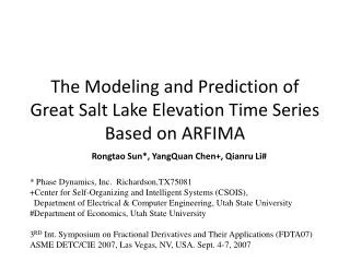
The Modeling and Prediction of Great Salt Lake Elevation Time Series Based on ARFIMA Rongtao Sun*, YangQuan Chen+, Qianru Li# * Phase Dynamics, Inc. Richardson,TX75081 +Center for Self-Organizing and Intelligent Systems (CSOIS), Department of Electrical & Computer Engineering, Utah State University #Department of Economics, Utah State University 3RD Int. Symposium on Fractional Derivatives and Their Applications (FDTA07) ASME DETC/CIE 2007, Las Vegas, NV, USA. Sept. 4-7, 2007
Applications to the Elevation Records of Great Salt Lake • The Great Salt Lake, located in Utah, U.S.A, is the fourth largest terminal lake in the world with drainage area of 90,000 km2. • The United States Geological Survey (USGS) has been collecting water-surface-elevation data from Great Salt Lake since 1875. • The modern era record-breaking rise of GSL level between 1982 and 1986 resulted in severe economic impact. The lake levels rose to a new historic high level of 4211:85 ft in 1986, 12.2 ft of this increase occurring after 1982. • The rise in the lake since 1982 had caused 285 million U.S. dollars worth of damage to lakeside. • According to the research in recent years, traditional time series analysis methods and models were found to be insufficient to describe adequately this dramatic rise and fall of GSL levels. • This opened up the possibility of investigating whether there is long-range dependence in GSL water-surface-elevation data so that we can apply FOSP to it.
Study area of Great Salt Lake • Adapted from M. Kemblowsli and Asefa, \Dynamic reconstruction of a chaotic system: The Great Salt Lake case," Utah Water Research Laboratory, Utah State University, 2003, working paper, 16p.
Long-term water-surface elevation graphs of the Great Salt Lake
Initial processing of GSL data • Let Itrepresents the levels of Great Salt Lake. We define rIas the logarithmic difference of the adjacent measurements. • Then, we define vIas the logarithmic of squared rI. • While the data set seems to be approximately uncorrelated, it is commonly accepted that they are not independent because the volatility clustering. • Log transformation reduces the skewness and makes unconditional distributions closer to the normal distribution.
Power spectral density of the volatility of GSL water-surface elevation
R/S Analysis • The R/S statistic is the range of partial sums of deviations of a time-series from its mean, rescaled by its standard deviation. A log-log plot of the R/S statistic versus the number of points of the aggregated series should be a straight line with the slope being an estimation of the Hurst exponent.
Aggregated Variance Method • The method plots in log-log scale the sample variance versus the block size of each aggregation level. If the series is long-range dependent then the plot is a line with slope greater than -1. The estimation of H is given by
Absolute Value Method • The log-log plot of the aggregation level versus the absolute first moment of the aggregated series is a straight line with slope of H -1, if the time series is long-range dependent.
Variance of Residuals Method • The method uses the least-squares method to fit a line to the partial sum of each block. A log-log plot of the aggregation level versus the average of the variance of the residuals after the fitting for each level should be a straight line with slope of H=2.
Periodogram Method • This method plots the logarithm of the spectral density of a time series versus the logarithm of the frequencies. The slope provides an estimate of H = 0.547.
Autoregressive fractional integral moving average (ARFIMA) • Using a fractional differencing operator which defined as an infinite binomial series expansion in powers of the backward-shift operator, we can generalize ARMA model to ARFIMA model. where L is the lag operator, are error terms which are generally assumed to be sampled from a normal distribution with zero mean:
ARFIMA Modeling and Forecasting • Standard deviations of the forecasting by ARFIMA with different samples for training
ARFIMA Modeling and Forecasting • Standard deviations of the forecasting by ARFIMA with different forecasted samples
ARFIMA Modeling and Forecasting • 2002-2007 GSL elevation differences forecasting
ARFIMA Modeling and Forecasting • 2002-2007 GSL elevation forecast by ARFIMA
Conclusions • Fractional order signal processing techniques are very useful in analyzing real world data and is developing incredibly fast. • Great Salt Lake data are found to have long-range dependence. • ARFIMA model has been successfully implemented for fitting the volatility of GSL water-surface-elevation data. It has been found to provide satisfactory forecast of the water-levels in the future. The experiments also show that more previous data samples result in better forecasting.