Download
1 / 59
910 likes | 1.81k Views
THE TRAVELING WAVE FAULT LOCATION OF TRANSMISSION LINE WAVELET TRANSFORM. Introduction . Locating transmission line faults quickly and accurately is very important for economy, safety and reliability of power system.

E N D
THE TRAVELING WAVE FAULT LOCATION OF TRANSMISSION LINE WAVELET TRANSFORM
Introduction • Locating transmission line faults quickly and accurately is very important for economy, safety and reliability of power system
This paper presents a recent fault location method based on the double terminal methods of traveling wave using WAVELT transform
Wavelet Transform has much better resolution for locating a transient event in time-domain over traditional methods such as fourier transform method.
In this presentation, some concentration will be upon transmission line system which is out point of interest in this project, especially the traveling wave theory.
Main power system components Any electric power system consists of three principal divisions: • generating system • transmission system • distribution system
transmission lines specifications & modeling • The transmission network is a high voltage network designed to carry power over long distances from generators to load points.
This transmission system consists of: • insulated wires or cables for transmission of power • transformers for converting from one voltage level to another • protective devices, such as circuit breakers, relays. • physical structures such as towers and substations
Any transmission line connecting two nodes may be represented by its basic parameters, namely • : • 1. Resistance (R) • 2. Inductance (L) • 3. Capacitance (C) • See next picture: pi-network
Transmission lines may be modeled as: • short lines ( < 80 km ) or • medium-length line ( 80 km < length < 240 km ) or • long lines ( > 240km )
Types of faults on Transmission lines: • The normal mode of operation of a power system is a balanced 3-phase AC. There are undesirable incidents that may disrupt normal conditions, as when the insulation of the system fails at any point. Then we say a fault occurs.
Protection schemes for transmission lines • The protection system is designed to disconnect the faulted system element automatically when the short circuit currents are high enough to present a direct danger to the element or to the system as a whole.
Any protection system consists of three principal components • sensor • protective relay • circuit breaker
There are two types of protection: • primary protection • backup protection
Faults may be classified under four types: • single line-to-ground fault SLG • line-to-line fault L-L • double line-to-ground fault 2LG • balanced three-phase fault
Fault detection methods in transmission lines Some of the fault location techniques Several fault location algorithms based on one-terminal have developed since several years ago.
They can be divided into two categories: • algorithm based on impedance in last years • algorithm based on traveling wave
algorithm based on impedance • uses current and voltage sampling data to measure post-fault impedance. Based on the knowledge of line impedance per unit length, the fault distance can be calculated.
algorithm based on traveling wave • While in the later, traveling wave determines fault location with the time difference between initial wave and its reflection one's arrival at the point of fault locator.
Algorithms of fault location based on traveling waves • When a line fault occurs, abrupt change in voltage or in current at the fault point generates a high frequency electromagnetic signal called traveling wave. This traveling wave propagates along the line in both directions away from the fault point.
1) Single-ended fault location algorithm • Single terminal methods are that the fault point is calculated by the traveling time between the first arrival of the traveling wave and the second arrival of the reflection wave at end of the line.
1) Single-ended fault location algorithm • This time is proportional to the fault distance and the key is to analyze the reflection process of traveling wave. A correlation technique is used to recognize the surge returning from the fault point and distinguish it from other surges present on the system.
1) Single-ended fault location algorithm • The method is suitable for a typical long line, but surely is inadequate for a close-in fault only a few kilometers from the measuring point. It thinks of the different velocities of earth mode and aerial mode, but the fault location error is great for the velocity chosen is not reliable.
2) Double-ended fault location algorithm • The double terminals methods are that fault point is determined by accurately time tagging the arrival of traveling wave at each end of the line. This method depends less on grounding resistance and system running-way, etc... This method is used widely.
2) Double-ended fault location algorithm • The velocity is determined by the distributed parameters ABCD of the line and usually varies in the range 295-29m/us for 500 kV line. The accuracy is improved by right of higher frequency components of traveling wave generated by lighting strikes
Wavelet and its transform fundamentals • WT has become well known as a new useful tool for various signal-processing applications. The wavelet transform of a signal f(t)L2 ( R) is defined by the inner-product between ab(t) and f (t) as:
Features and properties 1) Mother wavelet • (t) is a basic wavelet or mother wavelet, which can be taken as a band-pass function (filter). • The asterisk denotes a complex conjugate, and a,b R, a=/ 0, are the dilation and translation parameters.
2) Scaling wavelet • In the previous wavelet function, the time remains continuous but time-scale parameters (b,a) are sampled on a so-called “dyadic” grid in the time-scale plane (b,a).
Therefore, instead of continuous dilation and translation the mother wavelet may be dilated and translated discretely by selecting appropriate values of a and b
Reconstruction of original signal • It is possible to perfectly recover the original signalf(t) from its coefficientsWf(a,b) The reconstructed signal is defined as:
Hence, Wavelets exist locally in both the domains of time and frequency, owing to the good localization and the dilation/translation operation
Analysis by orthogonal wavelets shows little hope for achieving good time localization. We study how to use CWT to solve the problems of fault location in transmission lines. It is very advantageous for expanding the applied fields of WT and improving safety and reliability of power system
Advantages of wavelet transformation over other conventional methods • Two fundamental tools in signal analysis are the Windowed (or short-time) Fourier Transform (WFT) and the CWT. Both methods decompose a signal by performing inner products with a collection of running analysis functions
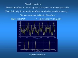
Fourier • For the WFT, the signal is decomposed into a summation of periodic and sinusoidal function. The time and frequency resolution are both fixed. That makes this approach particularly suitable for the analysis of signals with slowly varying periodic stationary characteristics. Hence, Fourier transform doesn’t indicate when an “event” occurs and doesn’t work well on discontinuous.
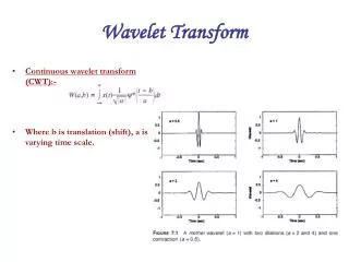
Wavelet • For the CWT, the analysis functions are obtained by dilation of a single (band-pass) wavelet. CWT uses short windows at high frequencies and long windows at low frequencies. This property enables the CWT to “zoom in” on discontinuous and makes it very attractive for the analysis of transient signals. The following figures are illustration of both method.
Wavelet applications areas • WT has been applied in • 1. signal processing • 2. power engineering
power engineering • analysis for power quality problems resolution • power system transient classification • power quality disturbance data compression and incipient failure detection.
Problem Formulation • consider our previous double-ended line • Lossless line, characteristic impedance Zc
Assume the traveling wave velocity of v. • if a fault occurs at a distance l1 from bus A, this will appear as an abrupt injection at the fault point. This injection will travel like a wave "surge" along the line in both directions and will continue to bounce back and forth between fault point, and the two terminal buses until the post-fault steady state is reached.
Using the knowledge of the velocity of traveling waves v along the given line, the distance to the fault point can be deduced easily
Proposed Method Analysis • Fault type: 3-phase fault • Algorithm: The double-ended line recording of fault signals method is used at both ends. • The recorded waveforms will be transformed into modal signals. • Fault locator method: The modal signals will be analyzed using their wavelet transforms..
Let t1 and t2 corresponds to the times at which the modal signals wavelet coefficients in scale 1, show their initial peaks for signals recorder at bus A and bus B. the delay between the fault detection times at the two ends is t1-t2, can be determined. When td is determined we could obtain the fault location from bus A According to: