Download
1 / 31
1.12k likes | 6.25k Views
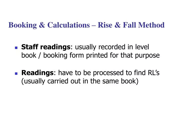
Booking & Calculations – Rise & Fall Method. Staff readings : usually recorded in level book / booking form printed for that purpose Readings : have to be processed to find RL’s (usually carried out in the same book).

E N D
Booking & Calculations – Rise & Fall Method • Staff readings: usually recorded in level book / booking form printed for that purpose • Readings: have to be processed to find RL’s (usually carried out in the same book)
Recommended: hand-held calculator / notebook computer with spreadsheet: avoid hand calculations & potential mistakes • Rise & fall method: one of most common booking methods • all rise/falls computed & recorded on sheet • RL of any new station: add rise to (or subtract fall from) previous station’s RL, starting from known BM.
Example 1.Rise & fall method (staff readings in Fig. 2.12): Table 2.2: 2.518 3.729 0.556 4.153 4.212 0.718 B CP2 Fig. 2.12 CP1 Table 2.2 BM
From (2.3), (2.4) & (2.5), = Total rise – total fall = Last RL – first RL Equalities checked in last row of Table 2.2. Any discrepancy existence of arithmetic mistake(s), but has nothing to do with accuracy of measurements.
Example 2.BS, FS (& IS) readings in Fig. 2.13 are booked as shown in Table 2.3: 0.595 1.522 2.234 3.132 2.587 1.985 1.334 TBM 2.002 58.331m above MSL B A C D Fig. 2.13 BS & FS Observed at Stations A - D Table 2.3 Using rise & fall method, a spreadsheet can be written to deduce RLs of points A through D as shown in Table 2.4. (use IF & MAX in Excel): you are encouraged to reproduce Table 2.4 on Excel.
Table 2.4 Last row of Table 2.4 = Total rise – total fall = Last RL – first RL no mistake with arithmetic.
Closure Error • Definition of misclosure & allowable values • Whenever possible: close on either starting benchmark or another benchmark to check accuracy & detect blunders. Misclosure (evaluated at closing BM): = measured RL of BM correct RL of BM (2.9) If acceptable: corrected for so that closing BM has correct known RL
Max. acceptable misclosure (in mm): E = C • where K = total distance of leveling route (in number of kilometers) C = a constant: typically between 2 mm (precise leveling work of highest standards) & 12 mm (ordinary engineering leveling)
Somewhat empirical values; can be justified by statistical theory; Bannister et al. (1998). • Construction leveling: often involves relatively short distances yet a large number (n) of instrument stations. In this case, an alternative criterion for E can be used: E = D (2.10) 5 mm & 8 mm: commonly adopted values for D.
LS Adjustment of Leveling Networks Using Spreadsheets Surveyors: often include redundancy Fig. 2.15: leveling network & associated data Arrowheads: direction of leveling; e.g. Along line 1: rise of 5.102 m from BM A to station X, i.e. RLX – RLA = 5.102, Along line 3: fall of 1.253 m from B to Z, i.e. RLZ – RLB = –1.253. (unknown) RLs of stations X, Y, Z: lower-case letters x, y, z. Fig. 2.15
Common practice in leveling adjustments: observations assigned weights inversely proportional to (plan) sight distances L: wi=(2.11) i = 1, 2, …, 7. • Objective: determine x, y, z. Many different solutions (e.g. by loop A-X-Y-Z-A, or B-Z-Y-X-B), probably all differ slightly random errors in data.
Utilize all available data & weights: least squares analysis. • Note: 7 observed elevation differences: vector [x – 200.000,207.500 – x, z – 207.500, 200.000 – z, y – x, y – 207.500, z – y]T
This vector can be decomposed into a matrix product as follows: (2.12)
Separate unknowns from constants re-write leveling information Ax+ k1 ~ k2 where A = coefficient matrix of 0’s & 1’s on RHS of (2.12), k1 = last vector in (2.12) containing benchmark values, k2= [5.102, 2.345, -1.253, -6.132, -0.683, -3.002, 1.703]T. Problem now in “Ax ~ k” form, where k = k2 – k1, weight matrix W = Diag [1/40,1/30,1/30,1/30,1/20,1/20,1/20]
Problem treated in Ch.1: • Solution: (1.5) numerical matrix computations • Spreadsheet method: • fast, easy to learn, highly portable • instant, automatic recalc. if #s in problem changed (common situation in surveying updating of control coordinates, discovery of mistakes, etc.).
Spreadsheet: shown in Table 2.6. Note: • computed #s in Table 2.6: do not necessarily show all d.p. paper space limitations (all computations: full accuracy). • Format – Cells – Number – Decimal places to display only desired number of d.p. (computations always carry full accuracy). • Select any cell in matrix ctrl - * whole matrix selected (matrix must be completely surrounded by blank border) See Table 2.6steps to be carried out on spreadsheet:
Table 2.6 Performing LS Adjustment of Leveling Network on a Spreadsheet Most probable RL’s for stations X, Y, Z: 205.148 m, 204.482 m, 206.188 m, respectively.
Contours • Contour lines:best method to show height variations on a plan • Contour line drawn on a plan: • a line joining equal altitudes • Elevations: indicated on plan • “tidemarks left by a flood” that fell at a discrete contour interval.
Fig. 2.16: plan & section of an island • contour line of 0 meter value: “tidemark left by the sea” • Ascending at 10 m contour intervals: a series of imaginary horizontal planes passing through island contours with values of 10 m, 20 m, 30 m, & 40 m, at their points of contact with island.
Fig. 2.16 gradient of the ground between A & C: • Gradient along AC = = 1 in 6 • Similarly, • Gradient along DE = = 1 in 3 • regions where contours are more closely packed have steeper slopes • a contour line is continuous & closed on itself, although the plan may not have sufficient room to show. • Height of any point: unique two contour lines of different values cannot cross or meet, except for a cliff / overhang.
Contouring: laborious. One direct method: • BM (30.500 m above HKPD) sighted, back sight = 0.500 m height of instrument (HI) = 31.000m. • Staff reading = 1.000 m staff’s bottom at 30-m contour level • Staff then taken throughout site, and at every 1.000 m reading, point is pegged for subsequent determination of its E, N coordinates by another appropriate survey technique 30-m contour located. • Similarly, a staff reading = 2.000 m a point on 9-m contour & so on. • Tedious & uneconomical for large area • Suitable in construction projects requiring excavation to a specific single contour line.
P Tall Building vertical line h Z B’ V horizontal line A (instrument center) B G Fig. 2.17 Trigonometric Leveling Discussion so far: differential leveling: may not be practical for large elevations (e.g. tall building’s height) trigonometric leveling( “heighting”): basic procedure:
rough estimate of h, e.g. residential buildings: h (number of stories 3 m). • Useful for checking result later, also a good separation (if possible) between instrument & building (why?). • If taping: horizontal distance AB from instrument to building obtained directly. Alternatively: EDM at A + reflector at some point B’ directly above / below Bslope distance AB’ & zenith angle AB & B’B computed. Also, vertical distance BG (or prism height B’G) to base of building: by a staff / tape.
Raise telescope to sight building top, measure v precisely. • Note: most theodolites give zenith angle z, vertical angle = v = 90 – z. Height of building: PG = AB tan v + BG (where BG = B’G – B’B if EDM was used).
Modern Instruments • Many total stations:built-in Remote Elevation Measurement (REM) mode expedites trigonometric leveling: • Sight point B’ (Fig. 2.17) once; distance & zenith angle measured & stored. • As one raises / lowers telescope corresponding height of new sighted point calculated & displayed automatically. Reflector to be placed at B’ (usually: prism on top of a held pole)
Difficulties: • People walking outside base of building may block prism: • Reflectorless total station: EDM laser beam can be reflected back from suitable building surfaces (e.g. white walls) w/o prism. Fig. 2.18(b) can sight any convenient point B’ along PG (see Fig. 2.17) w/o prism, • Only limitations: laser’s maximum range (typically ~ 100 m) & type of building’s surface (certain absorbing/ dark surfaces may not work).
Sighting top of tall building steep vertical angles telescope points almost straight up reading eyepiece becomes difficult to view: • Diagonal eyepiece: provides extension of eyepiece & allows comfortable viewing from the side: Fig. 2.18(a). (a) A Diagonal Eyepiece (b) Nikon NPL-820 Reflectorless Total Station Fig. 2.18 Leveling fieldwork: time-consuming & error-prone, especially for staff reading by eye.
Digital levels (DL): • capable of electronic image processing. • Require specially made staffs with bar codes on one side & conventional graduations on the other. • Observer directs telescope onto staff’s bar-coded side & focuses on it, as done in conventional leveling. • By pressing a key: DL reads bar codes & determines corresponding staff reading, displaying result on a panel. • Eliminate booking errors & expedite leveling work • Can be used in conventional way also.
Standard error for DL:typically < 1 mm at a sighting distance = 100 m Observation range:typical upper limit ~ 100 m, lower limit ~ 2 m. (a) Topcon DL-103 Digital Level (b) Bar-coded side of a staff Fig. 2.19