Download

1 / 33
330 likes | 535 Views
Maximum Test Coverage Minimum Test Cases. Using Equivalence Classes to your advantage. Introduction. John Arrowwood – john@irie-inc.com Been doing QA in the Portland area since 1996 Certified ScrumMaster , working on Agile teams since 2007 Specialize in test automation

E N D
Maximum Test Coverage Minimum Test Cases Using Equivalence Classes to your advantage
Introduction • John Arrowwood – john@irie-inc.com • Been doing QA in the Portland area since 1996 • Certified ScrumMaster, working on Agile teams since 2007 • Specialize in test automation • Have worked as a consultant for a plethora of companies: Intel, Regence, TransUnion, Dynamics Research Corp (Amdocs), RuleSpace, Merant (Serena), CenturyTel, Iovation, Windstream Communications, and Kronos. Current contract is with the IVR team at Comcast
The Problem • More and more, applications are database-driven • The size of those databases keeps getting bigger • The behavior of the application depends on the characteristics of the data • How much testing is “enough?”
How Much is Enough? • Test as much as you can before ship date • Beat on it until the incoming defect rate falls below some arbitrary threshold • Gut Feel – can we ship it? • Test Plan 100% executed • The open question for all of these is: • Have we tested enough to find all significant defects? • What haven’t we tested?
Example • Service Function • Regence – Out of Pocket Calculator • Output depends on Input • Countless permutations of inputs are possible • Customer – location, plan details, deductable met? • Provider – in network, out of network, agreements • Service – specific procedure being provided • Which customers do I need to test? • Which Providers should I test with?
A Simpler Example • Database of people • TransUnion – Consumer Lookup – Credit Report • Regence – Provider Search • Testing functionality: lookup by last name • Requirement: All records are findable • Example searches: smith, zeta-jones, de la joya, o’conner • What else do I need to test? • Are there other names I should try?
Option 1: Test Everything • If time allowed, this would be the ideal solution, as no defect would be left un-discovered • But for any realistic data set size, this is unfeasible • 375 million records at TransUnion • At one per second, average, would take almost 12 years to test them all • And that is without testing any variations and permutations of the search criteria • And because of the redundancy in the data, many of those tests would be a waste of effort, anyway
Data Redundancy • There is a lot of redundancy in real-world data sets • In the 1990 US Census, over 1% of the population has a last name of Smith. • The ten most popular last names make up over 5.5% of the population • Over 2.5% of women are named Mary • The top 10 names make up almost 11% of women • 3.3% of men are named James, another 3.2% are John, and the top ten names make up 23% of all men! • Just how many guys are there named “John Smith” ??? • Time spent testing redundant test cases is wasted
Option 2: Random Sample Set • Common for very large data sets, like at TransUnion • Gives a (supposedly) reasonable approximation correctness and predictability • With a 2 week test cycle, at best, test 1.2 million records at one per second • That is 0.32% • Business wanted any characteristic that appears in at least 5% of data to be tested • A lot of characteristics above that threshold would most likely never get tested! • Data redundancy • If 1% of whole set is Smith, then 1% of random subset probably is, too • You spend around 3-1/2 hours of your limited 2 weeks testing Smith records, when you really only needed to spend 1 second testing one of them
Option 3: Hand-Selection • A domain or subject-matter expert (SME) - maybe you, maybe not - can select your test cases • You are unlikely to select redundant test cases, so you can be more efficient • Are you certain you have tested everything that needs to be tested? • 375 million records condensed to 64 million distinct surnames • Never would have guessed that the data set included strange things like “surname(nickname)” or “a.surname” • Manual review of the 64 million names never revealed them
Option 4: Equivalence Classes • Analyze the production data, and iteratively and programmatically assign records to buckets, where every record in the bucket is interchangeable for any other • When you are done, you test one record per bucket • If properly defined, you can test exactly enough to prove correctness, no more, no less • Think of it as a SME on steroids – it has the patience and tenacity to analyze billions of records • But it is only as correct as the logic put into it
Equivalence Classes • Mathematically, an equivalence class is all values of x which, when input into the function f(x), evaluate to the same output value y • See http://en.wikipedia.org/wiki/Equivalence_class • In Quality Assurance, an Equivalence Class is the set of all inputs that can be seen as interchangeable with one another without impacting the results of the test, where only one of them needs to be tested in order to have confidence in the test results • See http://en.wikipedia.org/wiki/Equivalence_Partitioning
Example Partitions • Valid vs. Invalid input values • Upper-bound, lower-bound, in-bound, out-of-bounds • Empty-set vs. one, two, or three or more elements • Empty input vs. normal, vs. max-size, vs. oversize • Can you name others?
Pre-Requisites • Equivalence Partitioning doesn’t require coding ability • Figuring out how best to partition millions of records does • It’s worth the investment to obtain those skills, or hire someone who has them, or conscript a developer into doing this work • The production data must be available for programmatic analysis – preferably in a readily accessible format, e.g. .csv or .xml • Barring that, maybe extract data from production logs • You must have the computational resources to do the analysis
Example: Surnames • Database with 375 million distinct people in it • 64 million distinct last names • Top 90 percentile are equivalent • Built a histogram of surnames, most common first • Manually reviewed this list • Quickly determined that it was still too many to go through
Data Patterns • Converted every name to a pattern: • Converted every upper-case letter to ‘A’ • Every lower-case letter to ‘a’ • And every digit to ‘9’ • Generated a new histogram – count, pattern, example • List was smaller, but still too big • And there were still a lot of clearly equivalent test cases • But, now I started to see some of the oddball things showing up in the list
Visual Raw Histogram Pattern Histogram 55016653Aaaaaa Miller 44526736Aaaaa Smith 44043929Aaaaaaa Johnson 28721375Aaaaaaaa Williams 20727790Aaaa Hall 14237549Aaaaaaaaa Rodriguez 6060133Aaaaaaaaaa Richardson 3531179Aaa Lee 2216343Aaaaaaaaaaa Christensen 686906Aaaaaaaaaaaa Christiansen 519600Aa Le 448141AaAaaaaa McDonald 360436AaAaaaa McGuire 273971AaAaaa McLean 226265Aaaaaaaaaaaaa Hollingsworth 212366AaAaaaaaa McCormick 179730AaAaaaa De Jesus 137740AaAaaaaa Mc Donald 2069309 Smith 1629150 Johnson 1357432 Williams 1216138 Brown 1212358 Jones 955441 Miller 948214 Davis 685084 Wilson 670050 Anderson 631897 Taylor 625351 Thomas 615815 Garcia 613769 Moore 594073 Jackson 577366 Rodriguez
Incremental Improvement Previous Longer than 4 = equivalent 195839605 Aaaaa Smith 20727790Aaaa Hall 90% 3531179 Aaa Lee 1132856 AaAaaaa McDonald 972866AaaaaAaaaa Rivera Rivera 519600Aa Le 436146AaAaaaa De Jesus 339588Aaaaa-Aaaaa Pierre-Louis 286533A'Aaaaa O'Brien 273971AaAaaa McLean 240705Aaaaa-aaaa Pierre-louis99% 215607A'aaaaO'brien 186674AaaAaaaa Del Valle 133223AaAaaa De Leon 116553AaaaaAaaa Santa Cruz 116168AaAaa McCoy 113526AaaaAaaaa Diaz Rivera 103296 A M 55016653 Aaaaaa Miller 44526736 Aaaaa Smith 44043929 Aaaaaaa Johnson 28721375 Aaaaaaaa Williams 20727790 Aaaa Hall 14237549 Aaaaaaaaa Rodriguez 6060133 Aaaaaaaaaa Richardson 3531179 Aaa Lee 2216343 Aaaaaaaaaaa Christensen 686906 Aaaaaaaaaaaa Christiansen 519600 Aa Le 448141 AaAaaaaa McDonald 360436 AaAaaaa McGuire 273971 AaAaaa McLean 226265 Aaaaaaaaaaaaa Hollingsworth 212366 AaAaaaaaa McCormick 179730 AaAaaaaDe Jesus 137740 AaAaaaaaMc Donald
Iterative Process • Made the pattern function more and more complicated • Downloaded lists of names from census data, USPS, etc. • Tokenized the name, and for each token, if it matched one of the names in one of the lists, I replaced it with {list-name}, e.g. {surname}, {male}, {female}, {ambig}, {city}, {state}, etc. • If a token was not recognized, then the old pattern was the fall-back • Punctuation was never transformed, so it could be taken into account • After several iterative improvements, got the histogram down to about 38k patterns • Still too much to test manually, but perfectly reasonable for use in an automated test suite, if I were so inclined – testing could complete in under 11 hours • Equates to 0.01% of full data set, or 0.05% of full list of surnames • The top 95% were encompassed in the first 23 patterns in the list! • But upon inspection, there were clearly common elements farther down in the list, but I was able to justify where to stop the testing
Generalized Process • Get access to an extract of the raw data • Create f(x) • Always start simple, for example: s/[A-Z]/A/g; s/[a-z]/a/g; s/[0-9]/9/g; • Build a histogram showing the count, the pattern, and the most common input data that produced that pattern • Review this histogram (perhaps with the developers), decide which elements in the top few hundred are equivalent and which are not • Make intelligent changes to your transformation function to classify more equivalent values into the same bucket • Repeat until you are satisfied with the results
Example: Phonetic Encoding • SoundEx is one example of a phonetic algorithm that aims to put surnames that sound the same in the same bucket, ignoring variants of spelling • Smith, Smyth, Smythe would all fall in the same bucket • Bare, Bear, Bahr, and maybe even Beer, too • http://en.wikipedia.org/wiki/SoundEx • Other examples which aim to increase accuracy are • http://en.wikipedia.org/wiki/Metaphone • http://en.wikipedia.org/wiki/Match_Rating_Approach • http://en.wikipedia.org/wiki/New_York_State_Identification_and_Intelligence_System • TransUnion had their own, unpublished algorithm • All of these are excellent examples of the concept: a data transformation function which maps input values that are conceptually the same into a common output value
Example: Address • Given addresses: line1, line2, city, state, zip, plus4 • Due to the nature of the application, you should test at least one record per zip code • Because you can search by city+statewithout zip, you really need one per city+state+zip
Example: Address • If the application has custom parsing for the line1, you need an equivalence class function for it • Different cities have different address formats • 123 SW Main St • 123 Main St SW • 123 S Main St W • Some addresses will have apartment/suite information in line1, others in line2 • If the parsing of those fields is handled by a third party library, and you have the data in separate fields in your database, then you can probably ignore that field
Example: line1 Pattern • 123 SW Main St 19754 North East Broadway Boulevard • My Equivalence Class function • Tokenize the string • Using a defined priority, map recognized words into token class identifiers • With some, merge repeated token classes into one • Output for both: • {digits} {dir} {token} {tfare}
The Whole Record • For every field, you need to be able to have a custom function f(x) that handles that type of data • Some of those fields may use the same function, e.g. ec_enum(x) which returns the input value converted to lower case • You can choose to ignore some fields (e.g. plus4) • Always ignore volatile fields, like auto-increment primary keys, full phone numbers, etc. • Other fields are only relevant in combination with others (e.g. city, state, zip) • You want • an example of each distinct pattern for line1+line2 • an example of each city, state, zip combination • You do NOT want every pattern of line1 for each city, state, zip, as that would be hugely wasteful • But you would like your line1 patterns to be spread out over every city, state, zip combination
Getting What You Want • The process is the same as with the Surnames – the only difference is you don’t generate a single pattern • You generate one pattern for the line1 and line2 fields • You generate another for the city, state, zip • Associate the record with both patterns • Rather than having a single pattern that represents the data, you have two • The pattern string includes the context:$pattern_addr = ‘addr:’ . ec_address_pattern( line1, line2 );$pattern_csz = ‘csz:’. ec_city_state_zip( city, state, zip ); • Save both patterns in your histogram hash • Save a reference to the record for both pattern strings in your “example” mapping
The Magic Filter • In general, you process records as a filter • Keep a master hash table • key = pattern, value = reference to record • If frequency matters to you, keep another hash table • key = pattern, value = count of occurrences • Process records one at a time • Pass the record to your f(x) transformation function • For every pattern returned by your trans. function, update your hash tables (or update them directly in the function) • When you get to the end, you output all of the unique records still being pointed to by the master hash table
The Magic Filter • The part that does the actual filtering can be abstracted into reusable code • How it works: • In a modern language, objects/variables no longer being referenced are garbage collected • Your code stores a reference in the hash • As long as that reference remains, the record remains • When the last reference to that record is replaced by a reference to some other record that matches the same pattern, the redundant record is forgotten, and the memory it used is reclaimed for future records
Memory Constrained • This algorithm assumes that you have enough memory to store all of your selected test records • If that is not the case • Just keep a hash of all patterns that have been seen • If the record returned any “new” patterns, output it • Then add the “new” pattern to the hash for next time • This will be less than optimal, but it will allow you to filter to significantly fewer records without having to use as much memory to do it • NOTE: It is better to just get more memory, and use the memory you have wisely!
Normalized Data • What if the data is normalized? • Zero or more phone numbers? • Zero or more addresses? • Need to find a way to export it so that your filter can read it, e.g. xml • Add additional patterns, one or two per address, one per phone number, plus one to indicate how many addresses and another for how many phone numbers the record had
Statistical Skew • When using a randomly sampled subset of the data of sufficient size, you can usually infer or generalize something about the behavior of the data set as a whole • EC selection de-emphasizes common data elements, and over-emphasizes uncommon ones, completely destroying any ability to generalize based on your testing results • This technique is great for finding defects, not for characterizing the behavior of a system as a whole • Be aware and prepared to prevent anyone from trying to draw fallacious conclusions about the whole data set based on your testing of the subset
Determinism • Because of how the algorithm works, it will tend to select the last records seen, and only output older records that are not covered by more recent ones • This can create a statistical skew to the sample set (above and beyond the skew inherent to the algorithm) • It is best to process your records in random order • If you re-randomize, you then get different records • Otherwise, you will get the same set of records every time • This is an added insurance against your EC functions being inadequate
Questions? • FAQ: • Yes! You can email me if you have a question that we don’t get to here, and if time allows, I will answer it, no charge • Yes! Your organization can hire me for short-term engagements to help you implement these principles • Yes! It will not be cheap • Anything else?