Download
1 / 11
120 likes | 263 Views
Test Coverage. We have studied various black box and white box test techniques involving boundary values and test paths. Various “Quality Goals” may be articulated with test cases: 100% of input variables are boundary value tested 100% of code statements are executed

E N D
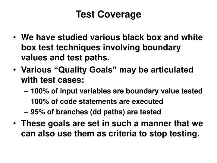
Test Coverage • We have studied various black box and white box test techniques involving boundary values and test paths. • Various “Quality Goals” may be articulated with test cases: • 100% of input variables are boundary value tested • 100% of code statements are executed • 95% of branches (dd paths) are tested • These goals are set in such a manner that we can also use them as criteria to stop testing.
Test Result Analysis accumulative # of defects found Slow down testing? More testing ! test time Number of problems found tend to slow down at some point in the over-all testing - - - that point is known as the “knee” of the curve when we start considering stopping the test.
“Buggy” Areas • There have been historical data that shows the “buggy” areas tend to be buggy all the way through the development life cycle (from review/inspection results of requirements to design to code through testing of code). • Also there has been historical indication that the code that has a large number of defects at the beginning of test tend to have a high probability of having a lot more defects. probability of more defects exist the higher the number of defects found in a module, the more likely it contains more defects!! balance against finding more bugs will clean up the module # of problems found in a module
What to focus on and When to end testing • After monitoring the test results, one might consider: • Testing more in the “buggy” code areas • Continue testing until the slowing down “knee” starts to appear. (tracking the test results also allows one to re-adjust the test schedule if necessary ---- very hard fight because testing is the last major activity before release)
Fault/Defect seeding • Since we can never be sure that all the defects are found and fixed, we are looking for indicators such as the testing “knee” to help us determine when to terminate testing. • Another methodology is to “seed” the code with defects: • Compare the number of seeded defects found against the total number of seeded defects. • Stop testing stop testing when that ratio is an “acceptable quality” level for the organization. • The key question is what type of seeded defects should one put in where: • Look at the history of defects of similar software produced by similar groups • Look at the early defects found in the “buggy” code areas - - - insert more seeded defects in those buggy areas.
Example of Defect Seeding • Suppose we decided to generate 50 seeded defects and insert them into the code. • Further suppose, through testing, we have found 45 of these seeded defects along with 392 indigenous (original unseeded) defects. Assuming a linear relationship of seeded and unseeded defects, we can use the ratio: (detected seeded) / (total seeded) = (detected unseeded) / (total unseeded) to estimate the total number of indigenous or unseeded defects. For the example, we have: 45 / 50 = 392 / total unseeded total unseeded = 435.5 or 436 defects Estimated remaining defects in the code is 436-392 = 44 unseeded defects Question: Is 45/50 = .9 or 90% discovery rate good enough? What was the Testing and Quality Goal? Can you live with possibly 44 more bugs? Is your maintenance-support team ready?
Confidence in Software with Defect Seeding • Our confidence that there are N defects in the software can be tested with seeding of S defects and running the test until we find all S seeded defects. Further suppose we find n actual non-seeded defects. Then our confidence level (CL) of there are N non-seeded defects can be defined as: CL = 100%. if n > estimated N CL = S/(S – N + 1), if n < or = estimated N This looks a bit strange. ( Look at page 407 of your text book ) 1) We would always have to use S > or = N to maintain a positive CL. 2) As long as n < N, CL does not change. Won’t you be concerned if n got pretty close to N?
Confidence Level • With the previous example of seeding, we found 392 non-seeded defects. We estimated that there are a total of Z = 436 defects. • We claim that there are (436 – 392) = 44 defects remaining in the software. What is our confidence? • Let’s put in 44 seeded defects and run this software until we find all 44 seeded defects. • A) In the process assume we found 32 unseeded defects. Then our confidence level that estimated total remaining defects of N=44 is: • S = 44 and N = 44, with n=32 < N • CL = 44/ (44– 44 +1) = 44 / 1 = 44 % confidence level • B) Assume we found 1 unseeded defects. Then our confidence level that the estimated remaining defects of N=44 is: • n = 1 < N • CL = 44/ (44 – 44 +1) = 44% confidence level • C) Assume that we found 53 unseeded defects. Then our confidence level that there are N=44 defects is: • n = 53 > N = 44 • CL = 100% (Same: n= 1 or n = 32 !! ) Take a look at the “improved” formula for CL on page 408, taking into account that you may never find all the S seeded defect. Yes --- but not much better.
Multiple Team Testing of The Same Code • Only in very special cases can a software organization afford to use multiple teams to test the same code - - - (life critical?) • *** also assume that one group is just effective in finding defects in all parts of the code. Assume that there are 2 test groups, T1 and T2, who each have found x and y respectively from a potential of n defects in the code. Also there is a common number q from x and y that is the same set of defects in x and y. Then the effectiveness of T1 and T2 may be expressed as : E1 = x / n E2 = y / n If T1 is uniform in effectiveness in finding defects, then its effectiveness in finding those defects that T2 found is the same. So, for T1, x / n = q / y and for T2, y / n = q / x (** from a big assumption above) Then we have: E1 * E2 = (x / n) * (y / n) = (q / y) * (y / n) = q / n n = q / (E1*E2) = estimated total number of defects in the code
Example of 2 Teams testing • Consider T1 found 34 defects and T2 found 45 defects and there were 24 common defects found by both teams. So, E1 = 34 / n and E2 = 45 / n. But E1 is also 24/45 and E2 = 24/34 E1 = 24/45 = .533 = 53% effective E2 = 24/34 = .705 = 71% effective n = q / (E1 * E2) = 24/ (.53 * .71) = 24 / (.376) = 63.8 or 64 So we estimate that the total number of defects in the code is 64. T1 found 34 of the 64 and T2 found 45 of the 64. Does this satisfy the Quality Goal where T2 found estimated 71% of defects? There is an estimated of 64 – 45 = 19 more defects in the code. Is your support maintenance team ready for this many defects?
Where were the defects found? • Besides the numbers, we also know from before that “buggy” area tends to continue to be “buggy” - - - • So if the defects found tend to concentrate in certain areas, continue testing with a more stringent quality goal for those areas.