Download

1 / 67
670 likes | 677 Views
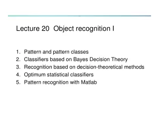
Object Recognition I. Linda Shapiro EE/CSE 576. Low- to High-Level. low-level. edge image. mid-level. consistent line clusters. high-level. Building Recognition. High-Level Computer Vision. Detection of classes of objects (faces, motorbikes, trees, cheetahs) in images

E N D
Object Recognition I Linda Shapiro EE/CSE 576
Low- to High-Level low-level edge image mid-level consistent line clusters high-level BuildingRecognition
High-Level Computer Vision • Detection of classes of objects (faces, motorbikes, trees, cheetahs) in images • Recognition of specific objects such as George Bush or machine part #45732 • Classification of images or parts of images for medical or scientific applications • Recognition of events in surveillance videos • Measurement of distances for robotics
High-level vision uses techniques from AI • Graph-Matching: A*, Constraint Satisfaction, Branch and Bound Search, Simulated Annealing • Learning Methodologies: Decision Trees, Neural Nets, SVMs, EM Classifier • Probabilistic Reasoning, Belief Propagation, Graphical Models
Graph Matching for Object Recognition • For each specific object, we have a geometric model. • The geometric model leads to a symbolic model in terms of image features and their spatial relationships. • An image is represented by all of its features and their spatial relationships. • This leads to a graph matching problem.
House Example 2D model 2D image L P RP and RL are connection relations. f(S1)=Sj f(S2)=Sa f(S3)=Sb f(S4)=Sn f(S5)=Si f(S6)=Sk f(S10)=Sf f(S11)=Sh f(S7)=Sg f(S8) = Sl f(S9)=Sd
But this is too simplistic • The model specifies all the features of the object that may appear in the image. • Some of them don’t appear at all, due to occlusion or failures at low or mid level. • Some of them are broken and not recognized. • Some of them are distorted. • Relationships don’t all hold.
TRIBORS: view class matching of polyhedral objects edges from image model overlayed improved location • Aview-class is a typical 2D view of a 3D object. • Each object had 4-5 view classes (hand selected). • The representation of a view class for matching included: - triplets of line segments visible in that class - the probability of detectability of each triplet The first version of this program used iterative-deepening A* search. STILL TOO MUCH OF A TOY PROBLEM.
RIO: Relational Indexing for Object Recognition • RIO worked with more complex parts that could have - planar surfaces - cylindrical surfaces - threads
Object Representation in RIO • 3D objects are represented by a 3D mesh and set of 2D view classes. • Each view class is represented by an attributed graph whose nodes are features and whose attributed edges are relationships. • For purposes of indexing, attributed graphs are stored as sets of 2-graphs, graphs with 2 nodes and 2 relationships. share an arc coaxial arc cluster ellipse
RIO Features ellipses coaxials coaxials-multi parallel lines junctions triples close and far L V Y Z U
RIO Relationships • share one arc • share one line • share two lines • coaxial • close at extremal points • bounding box encloses / enclosed by
Hexnut Object How are 1, 2, and 3 related? What other features and relationships can you find?
Graph and 2-Graph Representations 1 coaxials- multi encloses 1 1 2 3 2 3 3 2 encloses 2 ellipse e e e c encloses 3 parallel lines coaxial RDF!
Relational Indexing for Recognition Preprocessing (off-line) Phase for each model view Mi in the database • encodeeach 2-graph of Mi to produce an index • store Mi and associated information in the indexed bin of a hash table H
Matching (on-line) phase • Construct a relational (2-graph) description D for the scene • For each 2-graph G of D • Select the Mi’s with high votes as possible hypotheses • Verify or disprove via alignment, using the 3D meshes • encode it, producing an index to access the hash table H • cast a vote for each Mi in the associated bin
RIO Verifications incorrect hypothesis 1. The matched features of the hypothesized object are used to determine its pose. 2. The 3D mesh of the object is used to project all its features onto the image. 3. A verification procedure checks how well the object features line up with edges on the image.
Use of classifiers is big in computer vision today. • 2 Examples: • Rowley’s Face Detection using neural nets • Yi’s image classification using EM
Object Detection: Rowley’s Face Finder • convert to gray scale 2. normalize for lighting 3. histogram equalization 4. apply neural net(s) trained on 16K images What data is fed to the classifier? 32 x 32 windows in a pyramid structure
Object Class Recognition using Images of Abstract Regions Yi Li, Jeff A. Bilmes, and Linda G. Shapiro Department of Computer Science and Engineering Department of Electrical Engineering University of Washington
To solve: What object classes are present in new images ? ? ? ? Problem Statement Given: Some images and their corresponding descriptions {cheetah, trunk} {mountains, sky} {beach, sky, trees, water} {trees, grass, cherry trees}
Image Features for Object Recognition • Color • Texture • Context • Structure
Abstract Regions Line Clusters Original Images Color Regions Texture Regions
various different segmentations region attributes from several different types of regions Abstract Regions Multiple segmentations whose regions are not labeled; a list of labels is provided for each training image. image labels {sky, building}
Model Initial Estimation • Estimate the initial model of an object using all the region features from all images that contain the object Tree Sky
Final Model for “trees” Initial Model for “trees” EM Final Model for “sky” Initial Model for “sky” EM Classifier: the Idea
EM Algorithm • Start with K clusters, each represented by a probability distribution • Assuming a Gaussian or Normal distribution, each cluster is represented by its mean and variance (or covariance matrix) and has a weight. • Go through the training data and soft-assign it to each cluster. Do this by computing the probability that each training vector belongs to each cluster. • Using the results of the soft assignment, recompute the parameters of each cluster. • Perform the last 2 steps iteratively.
1-D EM with Gaussian Distributions • Each cluster Cj is represented by a Gaussian distribution N(j , j). • Initialization: For each cluster Cj initialize its mean j , variance j, and weight j. • With no other knowledge, use random means and variances and equal weights. N(1 , 1) 1 = P(C1) N(2 , 2) 2 = P(C2) N(3 , 3) 3 = P(C3)
Standard EM to EM Classifier • That’s the standard EM algorithm. • For n-dimensional data, the variance becomes a co-variance matrix, which changes the formulas slightly. • But we used an EM variant to produce a classifier. • The next slide indicates the differences between what we used and the standard.
EM Classifier • Fixed Gaussian components (one Gaussian per object class) and fixed weights corresponding to the frequencies of the corresponding objects in the training data. 2. Customized initialization uses only the training images that contain a particular object class to initialize its Gaussian. 3. Controlled expectation step ensures that a feature vector only contributes to the Gaussian components representing objects present in its training image. 4. Extra background component absorbs noise. Gaussian for Gaussian for Gaussian for Gaussian for trees buildings sky background
O1 O2 O1 O3 O2 O3 I1 I2 I3 W=0.5 W=0.5 W=0.5 W=0.5 W=0.5 W=0.5 W=0.5 W=0.5 W=0.5 W=0.5 W=0.5 W=0.5 1. Initialization Step (Example) Image & description
O1 O2 O1 O3 O2 O3 I1 I2 I3 W=0.8 W=0.2 W=0.2 W=0.8 W=0.2 W=0.8 W=0.8 W=0.2 W=0.8 W=0.2 W=0.2 W=0.8 2. Iteration Step (Example) E-Step M-Step
Object Model Database Color Regions Tree compare Sky p( tree| ) p( tree| ) p(tree | image) = f p( tree| ) p( tree| ) Recognition Test Image How do you decide if a particular object is in an image? To calculate p(tree | image) f is a function that combines probabilities from all the color regions in the image. e.g. max or mean
Combining different types of abstract regions: First Try • Treat the different types of regions independently and combine at the time of classification. • P(object| a1, a2,..,an) = P(object|a1)*..*P(object|an) • Form intersectionsof the different types of regions, creating smaller regions that have both color and texture properties for classification.
Experiments (on 860 images) • 18 keywords: mountains (30), orangutan (37), track (40), tree trunk (43), football field (43), beach (45), prairie grass (53), cherry tree (53), snow(54), zebra (56), polar bear (56), lion (71), water (76), chimpanzee (79), cheetah (112), sky (259), grass(272), tree (361). • A set of cross-validation experiments (80% as training set and the other 20% as test set) • The poorest results are on object classes “tree,”“grass,” and “water,” each of which has a high variance; a single Gaussian model is insufficient.
ROC Charts: True Positive vs. False Positive Independent Treatment of Color and Texture Using Intersections of Color and Texture Regions
Sample Retrieval Results cheetah
Sample Results (Cont.) grass
Sample Results (Cont.) cherry tree
Summary • Designed a set of abstract region features: color, texture, structure,. . . • Developed a new semi-supervised EM-like algorithm to recognize object classes in color photographic images of outdoor scenes; tested on 860 images. • Compared two different methods of combining different types of abstract regions. The intersection method had a higher performance
Weakness of the EM Classifier Approach • It did not generalize well to multiple features • It assumed that object classes could be modeled as Gaussians
Second Approach A Generative Discriminative Learning Algorithm for Image Classification Yi Li, Linda Shapiro, Jeff Bilmes ICCV 2005
A Better Approach to Combining Different Feature Types Phase 1: JUST CLUSTERING in features space • Treat each type of abstract region separately • For abstract region type a and for object class o, use the EM algorithm to construct clusters that are multivariate Gaussians over the features for type a regions.
Consider only abstract region type color (c) and object class object (o) • At the end of Phase 1, we can compute the distribution of color feature vectors in an image containing object o. • Mc is the number of components (clusters). • Thew’sare the weights (’s) of the components. • The µ’s and ∑’s are the parameters of the components. • N(Xc,cm,cm) specifies the probabilty that Xc belongs to a particular normal distribution.
Color Components for Class o component 1 component 2 component Mc µ1 ,∑1 , w1 µ2 ,∑2 , w2 µM ,∑M, wM r color feature vector Xc for region r
Now we can determine which components are likely to be present in an image. • The probability that the feature vector X from color region rof imageIi comes from component mis given by ? r Xci,r component m
And determine the probability that the whole image is related to component m as a function of the feature vectors of all its regions. • Then the probability that image Ii has a region that comes from component m is • where f is an aggregate function such as mean or max r1 X1 r2 P(X1,1) P(X2,1) P(X3,1) max component 1 component 2 X2 r3 X3
Aggregate Scores for Color Components 1 2 3 4 5 6 7 8 beach beach not beach