Download
1 / 49
490 likes | 628 Views
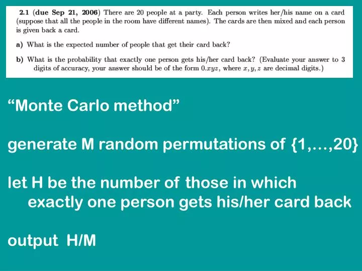
“Monte Carlo method” generate M random permutations of {1,…,20} let H be the number of those in which exactly one person gets his/her card back output H/M. Lower bounds. number from {1,2,3,…,9} 3 yes/no questions. Can you always figure out the number?. Lower bounds.

E N D
“Monte Carlo method” generate M random permutations of {1,…,20} let H be the number of those in which exactly one person gets his/her card back output H/M
Lower bounds number from {1,2,3,…,9} 3 yes/no questions Can you always figure out the number?
Lower bounds number from {1,2,3,…,8} 3 yes/no questions Can you always figure out the number?
Lower bounds number from {1,2,3,…,8} 3 yes/no questions in {1,2,3,4} ? Y N in {1,2} ? in {5,6} ? N N Y Y =7 ? =1 ? =3 ? =5 ? Y N Y N N Y Y N 7 8 3 4 5 6 1 2
Lower bounds number from {1,2,3,…,n} k yes/no questions
Lower bounds number from {1,2,3,…,n} k yes/no questions k = log2 n
Lower bounds number from {1,2,3,…,n} k yes/no questions k = log2 n INFORMATION THEORETIC LOWER BOUND: k log2 n
Lower bounds n animals = {dog,cat,fish,eagle,snake, …} yes/no questions INFORMATION THEORETIC LOWER BOUND: k log2 n
Lower bounds for sorting sorting by comparisons yes/no questions: is A[i]>A[j] ? data are not used to “control” computation in any other way A[1..n] • 1 2 3 • 1 3 2 • 2 1 3 • 3 1 • 3 1 2 • 3 2 1
Lower bounds for sorting sorting by comparisons yes/no questions: is A[i]>A[j] ? A[1..n] log a*b = log a + log b k log2 n! log2 n + log2 (n-1) + … log2 1 (n/2) log2 (n/2) = (n log n)
Lower bounds for sorting Theorem: Any comparison based sorting algorithm requires (n ln n) comparisons in the worst-case.
Lower bounds for search in sorted array INPUT: array A[1..n], element x OUTPUT: a position of x in A if x is in A otherwise
Lower bounds for search in sorted array INPUT: array A[1..n], element x OUTPUT: a position of x in A if x is in A otherwise Theorem: Any comparison based algorithm for searching an element in a sorted array requires (ln n) comparisons in the worst-case.
Lower bounds for minimum INPUT: array A[1..n] OUTPUT: the smallest element of A
Lower bounds for minimum INPUT: array A[1..n] OUTPUT: the smallest element of A INFORMATION THEORETIC LOWER BOUND: at least (ln n) comparisons ADVERSARY LOWER BOUND: at least (n) comparisons
Counting sort array A[1..n] containing numbers from {1,…,k} 1st pass: count how many times i {1,…,k} occurs 2nd pass: put the elements in B
Counting sort array A[1..n] containing numbers from {1,…,k} for i 1 to k do C[i] 0 for j 1 to n do C[A[j]]++ D[1]=0 for I 1 to k+1 do D[i+1] D[i]+C[i] for j 1 to n do D[A[j]]++ B[ D[A[j]] ] A[j]
Counting sort for i 1 to k do C[i] 0 for j 1 to n do C[A[j]]++ D[1]=1 for I 1 to k-1 do D[i+1] D[i]+C[i] for j 1 to n do B[ D[A[j]] ] A[j] D[A[j]]++ 1 2 3 2 2 4 2 1 1 2 3 3 2 1 2 4 C 4 7 3 2 D 1 5 12 15
Counting sort for i 1 to k do C[i] 0 for j 1 to n do C[A[j]]++ D[1]=1 for I 1 to k-1 do D[i+1] D[i]+C[i] for j 1 to n do B[ D[A[j]] ] A[j] D[A[j]]++ 1 2 3 2 2 4 2 1 1 2 3 3 2 1 2 4 C 4 7 3 2 D 2 5 12 15 1
Counting sort for i 1 to k do C[i] 0 for j 1 to n do C[A[j]]++ D[1]=1 for I 1 to k-1 do D[i+1] D[i]+C[i] for j 1 to n do B[ D[A[j]] ] A[j] D[A[j]]++ 1 2 3 2 2 4 2 1 1 2 3 3 2 1 2 4 C 4 7 3 2 D 2 6 12 15 1 2
Counting sort for i 1 to k do C[i] 0 for j 1 to n do C[A[j]]++ D[1]=1 for I 1 to k-1 do D[i+1] D[i]+C[i] for j 1 to n do B[ D[A[j]] ] A[j] D[A[j]]++ 1 2 3 2 2 4 2 1 1 2 3 3 2 1 2 4 C 4 7 3 2 D 2 6 13 15 1 2 3
Counting sort for i 1 to k do C[i] 0 for j 1 to n do C[A[j]]++ D[1]=1 for I 1 to k-1 do D[i+1] D[i]+C[i] for j 1 to n do B[ D[A[j]] ] A[j] D[A[j]]++ 1 2 3 2 2 4 2 1 1 2 3 3 2 1 2 4 C 4 7 3 2 D 2 7 13 15 1 2 2 3
Counting sort for i 1 to k do C[i] 0 for j 1 to n do C[A[j]]++ D[1]=1 for I 1 to k-1 do D[i+1] D[i]+C[i] for j 1 to n do B[ D[A[j]] ] A[j] D[A[j]]++ 1 2 3 2 2 4 2 1 1 2 3 3 2 1 2 4 C 4 7 3 2 D 5 12 15 17 1 1 1 1 2 2 2 2 2 2 2 3 3 4 3 4
Counting sort for i 1 to k do C[i] 0 for j 1 to n do C[A[j]]++ D[1]=1 for I 1 to k-1 do D[i+1] D[i]+C[i] for j 1 to n do B[ D[A[j]] ] A[j] D[A[j]]++ stable sort = after sorting the items with the same key don’t switch order running time = O(n+k)
Counting sort for i 1 to k do C[i] 0 for j 1 to n do C[A[j]]++ D[1]=1 for I 1 to k-1 do D[i+1] D[i]+C[i] for j 1 to n do B[ D[A[j]] ] A[j] D[A[j]]++ stable sort = after sorting the items with the same key don’t switch order running time = O(n+k) What if e.g., k = n2 ?
Radix sort array A[1..n] containing numbers from {0,…,k2 - 1} • sort using counting sort with • key = x mod k • 2) sort using counting sort with • key = x/k Running time = ?
Radix sort array A[1..n] containing numbers from {0,…,k2 - 1} • sort using counting sort with • key = x mod k • 2) sort using counting sort with • key = x/k Running time = O(n + k)
Radix sort array A[1..n] containing numbers from {0,…,k2 - 1} example k=10 28 21 42 43 23 32 70 18 29 20 70 20 21 42 32 43 23 28 18 29
Radix sort array A[1..n] containing numbers from {0,…,k2 - 1} example k=10 28 21 42 43 23 32 70 18 29 20 70 20 21 42 32 43 23 28 18 29
Radix sort array A[1..n] containing numbers from {0,…,k2 - 1} example k=10 28 21 42 43 23 32 70 18 29 20 70 20 21 42 32 43 23 28 18 29 18 20 21 23 28 29 32 42 43 70
Radix sort array A[1..n] containing numbers from {0,…,kd - 1} • sort using counting sort with • key = x mod k • 2) sort using counting sort with • key = x/k mod k • 3) sort using counting sort with • key = x/k2 mod k • … • d) sort using counting sort with • key = x/kd-1 mod k
Radix sort array A[1..n] containing numbers from {0,…,kd - 1} Correctness: after s-th step the numbers are sorted according to x mod ks Proof: By induction. Base case s=1 is trivial. 1) sort using counting sort with key = x mod k
Radix sort array A[1..n] containing numbers from {0,…,kd - 1} Correctness: after s-th step the numbers are sorted according to x mod ks Proof: Now assume IH and execute s+1st step. Let x,y be such that x mod ks+1 < y mod ks+1. Then either x/ks mod k < y/ks mod k or x/ks mod k = y/ks mod k and x mod ks < y mod ks
Bucket sort linear time sorting algorithm on average Assume some distribution on input. INPUT: n independently random numbers from the uniform distribution on the interval [0,1].
Bucket sort INPUT: n independently random numbers from the uniform distribution on the interval [0,1]. for i 1 to n do insert A[i] into list B[ A[i]*n ] for i 0 to n-1 do sort list B[i] output lists B[0],…,B[n-1]
Bucket sort INPUT: n independently random numbers from the uniform distribution on the interval [0,1]. 0.13, 0.23, 0.56, 0.74, 0.18, 0.34, 0.12, 0.82, 0.14, 0.19 for i 1 to n do insert A[i] into list B[ A[i]*n ] for i 0 to n-1 do sort list B[i] output lists B[0],…,B[n-1]
Bucket sort INPUT: n independently random numbers from the uniform distribution on the interval [0,1]. 0.13, 0.23, 0.56, 0.74, 0.18, 0.34, 0.12, 0.52, 0.14, 0.19 1 2 5 7 1 3 1 5 1 1 B[1]: 0.13, 0.18, 0.12, 0.14, 0.19 B[2]: 0.23 B[3]: 0.34 B[5]: 0.56, 0.52 B[7]: 0.74 for i 1 to n do insert A[i] into list B[ A[i]*n ] for i 0 to n-1 do sort list B[i] output lists B[0],…,B[n-1]
Bucket sort INPUT: n independently random numbers from the uniform distribution on the interval [0,1]. 0.13, 0.23, 0.56, 0.74, 0.18, 0.34, 0.12, 0.52, 0.14, 0.19 1 2 5 7 1 3 1 5 1 1 B[1]: 0.12, 0.13, 0.14, 0.18, 0.19 B[2]: 0.23 B[3]: 0.34 B[5]: 0.52, 0.56 B[7]: 0.74 for i 1 to n do insert A[i] into list B[ A[i]*n ] for i 0 to n-1 do sort list B[i] output lists B[0],…,B[n-1]
Bucket sort for i 1 to n do insert A[i] into list B[ A[i]*n ] for i 0 to n-1 do sort list B[i] output lists B[0],…,B[n-1] assume we use insert-sort worst-case running time?
Bucket sort for i 1 to n do insert A[i] into list B[ A[i]*n ] for i 0 to n-1 do sort list B[i] output lists B[0],…,B[n-1] assume we use insert-sort average-case running time? X0, X1, … , Xn-1 where Xi is the number of items that fall inside the i-th bucket
Bucket sort X0, X1, … , Xn-1 where Xi is the number of items that fall inside the i-th bucket X02 + X12 + … + Xn-12 What is E[X02 + X12 + … + Xn-12] ? linearity of expectation symmetry of the problem E[X02 + … + Xn-12 ] = E[X02] + … + E[Xn-12 ] = n E[X02]
Bucket sort E[X02] What is E[X0] ? p=1/n value of X0 • 0 (1-p)n • n (1-p) n-1 • k binomial(n,k) pk (1-p)n-k • n pn
Bucket sort p=1/n E[X02] E[X0] = 1 • 0 (1-p)n • n (1-p) n-1 • k binomial(n,k) pk (1-p)n-k • n pn n E[X0] = k * binomial(n,k) pk (1-p)n-k k=0
Bucket sort p=1/n E[X02] E[X0] = 1 n E[X0] = k * binomial(n,k) pk (1-p)n-k k=1 binomial (n,k) = (n/k) * binomial (n-1,k-1) binomial(n,k) pk (1-p)n-k = 1 n k=0
Bucket sort p=1/n E[X02] E[X0] = 1 n E[X0] = n* binomial(n-1,k-1) pk (1-p)n-k k=1 n = n*p binomial(n-1,k-1) pk-1(1-p)n-k = n*p k=1 binomial(n,k) pk (1-p)n-k = 1 n k=0
Bucket sort p=1/n E[X02] • 0 (1-p)n • n (1-p) n-1 • k binomial(n,k) pk (1-p)n-k • n pn n E[X02]= k2 * binomial(n,k) pk (1-p)n-k k=0
Bucket sort p=1/n E[X02] n E[X02]= k2 * binomial(n,k) pk (1-p)n-k k=0 n = k * binomial(n,k) pk (1-p)n-k k=0 n + k(k-1) * binomial(n,k) pk (1-p)n-k k=0
Bucket sort p=1/n E[X02] n E[X02]= k2 * binomial(n,k) pk (1-p)n-k k=0 n*p n = k * binomial(n,k) pk (1-p)n-k k=0 n + k(k-1) * binomial(n,k) pk (1-p)n-k k=0
Bucket sort p=1/n E[X02] n E[X02]= k(k-1) * binomial(n,k) pk (1-p)n-k +n*p k=2 binomial (n,k) = (n/k) * binomial (n-1,k-1) = (n/k) * ((n-1)/(k-1)) * binomial (n-2,k-2) E[X02] = n* (n-1) * p2 + n*p