Download
1 / 27
270 likes | 390 Views
Interpretation of station data with an adjoint Model. Maarten Krol (IMAU) Peter Bergamaschi (ISPRA) Jan Fokke Meierink, Henk Eskes (KNMI) Sander Houweling (SRON/IMAU). What is TM5?. Global model with zoom option Two-way nesting Mass-conserving / Positive

E N D
Interpretation of station data with an adjoint Model Maarten Krol (IMAU) Peter Bergamaschi (ISPRA) Jan Fokke Meierink, Henk Eskes (KNMI) Sander Houweling (SRON/IMAU)
What is TM5? • Global model with zoom option • Two-way nesting • Mass-conserving / Positive • Atmospheric chemistry Applications • Off-line ECMWF • Flexible geometry
What is TM5? 6x4 3x2 1x1
Why an Adjoint TM5? • Concentrations on a station depend on emissions • Interesting quantity: dM(x,t)/dE(I,J,t’) • How does a ‘station’ concentration at t changes as a function of emissions in gridbox (I,J) at time t’? • Inverse problem: from measurements M (x,t) --> E(I,J,t’)
Adjoint TM5 • dM(x, t)/dE(I,J) (constant emissions) can be calculated with the adjoint in one simulation • M0(x, t) = f(E0(I,J)) • M(x, t) = M0+dM(t)/dE(I,J)*(E(I,J)-E0(I,J)) • Only if the system is linear!
Finokalia MINOS 2001 measurements Dirty Clean
Finokalia • Integrations from M(t) back to july, 15. • Forcing at station rm(I,J,1) = rm(I,J,1) + f(t,t+dt) (during averaging period) • Adjoint chemistry • Adjoint emissions give analytically: dM(t)/dE(I,J)
Procedure • Minimise • With
Negatives Emissions over sea Posterior MCF emissions: BETTER CONSTRAIN THE PROBLEM
Conclusions • Emissions seem to come from regions around the black sea! • Results sensitive to prior information • Not surprising: 8 observations <==> 1300 unknowns • Emissions required: 10-30 gG/year • How to avoid negatives?
Next Steps (to be done) • Prior Information • non-negative • full covariance matrix • Full 4Dvar, starting with obtained solution as starting guess emissions • Influence station sampling, BL scheme, …. • All observations separately (Movie)