Download
1 / 41
490 likes | 739 Views
Radiation dosimetry for animals and plants. Jordi Vives i Batlle Centre for Ecology and Hydrology, Lancaster, 27 April 2010. Key concepts Kerma, absorbed dose, units, radiation weighting factor, absorbed fraction, dose conversion coefficient (DCC)

E N D
Radiation dosimetry for animals and plants JordiVivesiBatlleCentre for Ecology and Hydrology, Lancaster, 27 April 2010
Key concepts Kerma, absorbed dose, units, radiation weighting factor, absorbed fraction, dose conversion coefficient (DCC) ERICA approach to absorbed fraction calculation Reference habitats, organisms and shapes, Monte Carlo approach, sphericity, dependence with energy / size ERICA DCCs for internal and external exposure Internal and external DCC formulae, energy / size dependency, allometric scaling Comparing ERICA with other tools Special cases Gases, inhomogeneous sources, non-equilibrium Lecture plan
Kerma: sum of the initial kinetic energies of all the charged particles transferred to a target by non-charged ionising radiation, per unit mass Absorbed dose: total energy deposited in a target by ionising radiation, including secondary electrons, per unit mass Similar at low energy - Kerma am approximate upper limit to dose Different when calculating dose to a volume smaller than the range of secondary electrons generated Kerma and absorbed dose
Units of absorbed dose (Grays) = Energy deposited (J kg-1) Only small amounts of deposited energy from ionising radiation are required to produce biological harm - because of the means by which energy is deposited (ionisation and free radical formation) For example - drinking a cup of hot coffee transfers about 700 Joules of heat energy per kg to the body. To transfer the same amount of energy from ionising radiation would involve a dose of 700 Gy - but doses in the order of 1 Gy are fatal I Gy = 1 J kg-1 = 6.24 1015keV ~ 1012 alphas Units and significance
Need to make allowance of such factors as LET or RBE in the description of absorbed dose Equivalent dose = absorbed dose radiation weighting factor (wr) Units of equivalent dose are Sieverts (Sv) No firm consensus - suggested values for wr: 1 for and high energy (> 10keV) radiation 3 for low energy ( 10keV) radiation 10 for (non stochastic effects in the species) vs. 20 for humans (to cover stochastic effects of radiation i.e. cancer in an individual) Radiation weighting factor (wr)
Fraction of energy E emitted by a source absorbed within the target tissue / organism Internal and external exposures of an organism in a homogeneous medium: Dint = k Aorg(Bq kg-1) E (MeV) AF(E) Dext = k Amedium(Bq kg-1) E [1-AF(E)] k = 5.76 10-4 Gy h-1 per MeV Bq kg-1 If the radiation is not mono-energetic, then the above need to be summed over all the decay energies (spectrum) of the radionuclide Some models make simplifying assumptions: Infinitely large organism (internal exposure) Infinitely small organism (external exposure) Absorbed fraction (AF)
Defined as the ratio of dose rate per unit concentration in organism or the medium: Dint = k Aorg E AF(E) = DCCint Aorg Dext = k AmediumE[1-AF(E)] = DCCext Amedium Units of Gy h-1 per Bq kg-1 Concentration in organisms is concentration in the medium times a transfer function: Aorg =Amedium (t) In equilibrium, the transfer function is known as the “transfer factor”, TF Dose conversion coefficient (DCC)
The dose is the result of a complex interaction of energy, mass and the source - target geometry: Define organism mass and shape Consider exposure conditions (internal, external) Simulate radiation transport for mono-energetic photons and electrons: absorbed fractions Link calculations with nuclide-specific decay characteristics: Dose conversion coefficients Only a few organisms with simple geometry can be simulated explicitly In all other cases interpolation gives good accuracy Strategy for dose calculation
The enormous variability of biota requires the definition of reference organisms that represent: Plants and animals Different mass ranges Different habitats Exposure conditions are defined for different habitats: In soil/on soil In water/on water In sediment/interface water sediment Reference habitats & organisms
Reference organism shapes Organism shapes approximated by ellipsoids, spheres or cylinders of stated dimensions Homogeneous distribution of radionuclides within the organism: organs are not considered Oganism immersed in uniformly contaminated medium Dose rate averaged over organism volume
Monte Carlo approach Monte Carlo simulations of photon and electron transport through matter (ERICA uses MCNP code) Includes all processes: photoelectric absorption, Compton scattering, pair creation, fluorescence
Problems and limitations Monte Carlo calculations are very time-consuming: Long range of high-energy photons in air, a large area around the organism has to be considered A large contaminated area has to be considered as source Small targets get only relatively few hits Probability ~ 1/source-target distance2 Simulations require high number of photon tracks Therefore, a two-step method has been developed: KERMA calculated in air from different sources on or in soil Dose to organism / dose in air ratio calculated for the different organisms and energies
Spherical AFs vs. mass & energy Electrons Photons
Represented by ellipsoidal shapes having the same mass as the spherical ones AFs always less than those for spheres of equal mass. Non-sphericity parameter: = surface area of sphere of equal mass (S0) / surface area (S) Derive re-scaling factors RF using the formula: RF() can be approximated by a single-parameter curve: RF() = 1 for large masses and low energies, and for very small masses and high energies. Ulanovsky and Pröhl (2006) Non-spherical bodies
AF versus -energy Absorbed fractions for electrons in different terrestrial organisms (Brown et al., 2003)
For each radionuclide and reference organism energies and yields of all , and emissions are extracted from ICRP(1983) and overall and AF's calculated as: where Ei is energy (MeV) and pi denotes the fractional yield of individual emissions Overall AF for radionuclide
Calculation of dose rates • Internalexposure: • Externalexposure: • Occupancyfactor:
DCC for soil organisms DCCs for various soil organisms at a depth of 25 cm in soil for monoenergetic photons. Assumes uniformly contaminated upper 50 cm of soil (density: 1600 kg/m³) DCCs for earthworm at various soil depths for monoenergetic photons. Assumes uniformly contaminated upper 50 cm of soil
Energy dependence of DCCs DCCs for mono-energetic photons for soil organisms as a function of photon energy (Brown et al., 2003)
External DCCs decrease with size due to the increasing self-shielding, especially for low energy g-emitters Small organism DCCs from high-energy photons higher for underground organisms, & vice versa for larger organisms External exposure to low-energy emitters is higher for organisms above ground, due to lack of shielding by soil DCCs for internal exposure to -emitters (esp. high-energy) increase with mass due to the higher absorbed fractions For and -emitters, the DCCs for internal exposure are virtually size-independent DCCs versus size and energy
Allometric correlation with size • Vives i Batlle et al. (2004)
Intercomparison analysis International comparison of 7 models performed under the EMRAS project: EDEN, EA R&D 128, ERICA, DosDimEco, EPIC-DOSES3D, RESRAD-BIOTA, SÚJB 5 ERICA runs by different users: default DCCs, ICRP, SCK-CEN, ANSTO, K-Biota 67 radionuclides and 5 ICRP RAP geometries Internal doses: mostly within 25% around mean External doses: mostly within 10% around mean There are exceptions e.g.α and soft β-emitters reflecting variability in AF estimations (3H, 14C…) ERICA making predictions similar to other models
Internal dosimetry comparison Estimate ratio of average (ERICA) to average (rest of models) Skewed distribution centered at 1.1 Fraction < 0.75 = 40% Fraction > 1.25 = 3% Fraction between 0.75 and 1.25 = 57% • Worst offenders (< 0.25): 51Cr, 55Fe, 59Ni, 210Pb, 228Ra, 231Th and 241Pu • Worst offenders (>1.25): 14C, 228Th • Conclude reasonably tight fit (most data < 25% off)
External dosimetry comparison Same ratio method for external dose in water Two data groups at < 0.02 and ~ 1.32 Fraction < 0.5 = 37% Fraction > 1.5 = 13% Fraction between 0.5 and 1.5 =50 % Worst offenders (< 0.02): • 3H, 33P, 35S , 36Cl, 45Ca, 55Fe, 59,63Ni, 79Se, 135Cs, 210Po, 230Th, 234,238U, 238,239,241Pu, 242Cm • Worst offenders (>1.25): 32P, 54Mn, 58Co, 94,95Nb, 99Tc, 124Sb, 134,136Cs, 140Ba, 140La, 152,154Eu, 226Ra, 228Th • Still acceptable fit (main data < 50% “off”)
Approach for gases The following formulae can be used for radionuclides whose concentration is referenced to air: 3H, 14C, 32P, 35S, 41Ar and 85Kr
Inhomogeneous distribution () Tadpole Earthworm Frog Crab Duck Rat Central point Distributed source Eccentric point Trout Flatfish Deer Data from Gómez-Ros et al. (2009)
Inhomogeneous distribution () Tadpole Earthworm Frog Eccentric point Distributed source Crab Duck Rat Trout Flatfish Deer Central point Data from Gómez-Ros et al. (2009)
Argon and krypton Internal dose negligible: Ar and Kr CFs set to 0 No deposition but some migration into soil pores Assume pore air is at the same concentration as ground level air concentrations assume a free air space of 15%, density = 1500 kg m-3, so free air space = 10-4 m3 kg-1 & Bq m-3(air) * 10-4 = Bq kg-1 (wet) Hence, a TF of 10-4 for air (Bq m-3) to soil (Bq kg-1 wet) For plants and fungi occupancy factors set to 1.0 soil, 0.5 air (instead of 0) Biota in the subsurface soil and are exposed only to 41Ar and 85Kr in the air pore spaces External DCCs for fungi are those calculated for bacteria (i.e. infinite medium DCCs)
Radon dosimetry in biota At equilibrium: - iN R R+h L Conceptual representation of irradiated respiratory tissue Simple respiratory model for 222Rn daughters
Plants: breathing rate Use CO2 as analogue entering plant, while water and O2 exit through the stomata A full process dose model representing gas exchange through plant stomata is the next logical developmental step • Assume whole plant exchanges gases
Radon DCC derivation TB: Full tracheobronchial epithelium; L: Full lung; WB: Whole body; STBRM and SBRM : Area of tracheobronchial tree or bronchial epithelium; a: Axis of cylinder representing the plant; Rwfa:Weighting factor • Animal dose factors (Gy h-1 per Bq m-3): • Plant dose factors:
Each sub-model contains the decay chain of radon: 222Rn 218Po 214Pb 214Bi 214Po ICRP Radon model for plants
Non-equilibrium assessments Organisms can retain activity for a long time after it has been dispersed from an environment. Requires assessment tools based on a dynamic approach Time-dependent dose rates can be integrated over period following the intake of radioactivity (lifetime)
Brown J., Gomez-Ros J.-M., Jones, S.R., Pröhl, G., Taranenko, V., Thørring, H., Vives i Batlle, J. and Woodhead, D, (2003) Dosimetric models and data for assessing radiation exposures to biota. FASSET (Framework for Assessment of Environmental Impact) Deliverable 3 Report under Contract No FIGE-CT-2000-00102, G. Pröhl (Ed.). Gómez-Ros, J.M., Pröhl, G., Ulanovsky, A. and Lis, M. (2008). Uncertainties of internal dose assessment for animals and plants due to non-homogeneously distributed radionuclides. Journal of Environmental Radioactivity 99(9): 1449-1455. Ulanovsky, A. and Pröhl, G. (2006) A practical method for assessment of dose conversion coefficients for aquatic biota. Radiation and Environmental Biophysics 45: 20 -214. Vives i Batlle, J., Jones, S.R. and Gómez-Ros, J.M. (2004) A method for calculation of dose per unit concentration values for aquatic biota. Journal of Radiological Protection 24(4A): A13-A34. Vives i Batlle, J., Jones, S.R. and Copplestone, D. (2008) Dosimetric Model for Biota Exposure to Inhaled Radon Daughters. Environment Agency Science Report – SC060080, 34 pp. References