Download
1 / 23
230 likes | 349 Views
観測&装置ゼミ 第5回 2013.09.26 Weak field approximation. 発表者 渡邉皓子. 時代は E-book です. http://link.springer.com/book/10.1007/1-4020-2415-0/page/ 1 SPS-ID を入力すれば E-book が手に 入る “ Polarization in Spectral Lines ” E.Landi Degl’innocenti は名著です! 9.6 章 “ The Weak Field Approximation ” あたり が今回のトピック.

E N D
観測&装置ゼミ第5回2013.09.26Weak field approximation 発表者 渡邉皓子
時代はE-bookです • http://link.springer.com/book/10.1007/1-4020-2415-0/page/1 • SPS-IDを入力すればE-bookが手に入る • “Polarization in Spectral Lines”E.LandiDegl’innocentiは名著です! • 9.6章“The Weak Field Approximation”あたりが今回のトピック
時代は彩層磁場です • 飛騨天文台DSTでCa II K線でストークスパラメーターを観測する試みがあった(ですか?) • 私は今、Swedish Solar Telescope / CRISPのCa II K full Stokesデータを使っている • Solar-C でも彩層磁場を測る。そのラインの候補は、He I 10830, Ca II 8542, Hα 6563 http://hinode.nao.ac.jp/SOLAR-C/Meeting/SCSDM2/katsukawa2.pdf
弱磁場近似は光球でも • Solar Orbiter(2017-2018に打ち上げ予定で開発中)ではFe I 617.3nmを磁場測定に使う ←弱磁場近似を使って物理量を導く • 三鷹フレア望遠鏡では、Fe I 1564.8nmの太陽全面観測に対して、弱磁場近似を簡易的に用いることでマグネトグラムを開発中(参考:2013年9月天文学会での桜井先生資料)
2008年夏の清里宇宙天気サマースクールにおける、桜井先生の講義資料から重要点を抜粋しました2008年夏の清里宇宙天気サマースクールにおける、桜井先生の講義資料から重要点を抜粋しました • http://www.kwasan.kyoto-u.ac.jp/swss08/index.html(講義資料へのリンクが切れてる!)
When the Zeeman splitting is much smaller than the typical width of the profiles, it is possible to deduce some properties of the solutions to the transfer equation without actually solving it. The above condition means g vH << 1
weak field approximationを用いたマグネトグラムの作成(桜井先生資料より) • V = ΔλHcosθdI/dλ • ΔλH [nm]= 4.67 10-12geffλ[nm]2 B[gauss] • V /I=CL*BL フレア監視望遠鏡では、Fe 1564.8nmの Stokes line profileではなく、ラインセンター から0.4Åほと離れた部分でfiltergramを 撮っている
短波長のStokes V filtergramから、どうやってmagnetogramを作るか • Milne-Eddington大気のパラメータを調節して、磁場のないときの線輪郭を再現 • linear source function B=B0(1+βτ) • η(線吸収係数) • ΔλD(ドップラー幅) • a (damping constant) • 次に磁場を与えて海野の公式で偏光度を計算
mapを作る波長 Fe 1564.8 nm 1000 G くらいで偏光度最大 14% 磁場がすべて1kGとすれば、こちら→ CL=1.410-4 weak field approx.→ CL=6.010-5
フレア監視鏡のマグネトグラム作成は、まだ検討中とのことフレア監視鏡のマグネトグラム作成は、まだ検討中とのこと • SDOの磁場と比較→ CL=4.510-526 April 2010
I Q U V 私の研究ではこんな風に使っています line center MartínezGonzález & BellotRubio, 2009, ApJ 700, 1391
fitting結果サンプル 2540 Gauss 2470 Gauss
azimuthはこう出せる • E.Landi Degl’innocenti “Polarization in Spectral Lines” page 402 • for Q is not 0, U(λ)/Q(λ) = tan 2χ • 180 deg ambiguity is included and so, the result is -45deg to 45deg least-squareなら下記になるが、tangentの位相が第一象現になるので、 結果の値は0~45°の間しか取らない
inclinationにたどり着くまではちょっと複雑 注1:L(λ) = sqrt(Q(λ)^2 +U(λ)^2) 注2 : λ is the distance to line center
Lande factor 表 • http://hinode.nao.ac.jp/SOLAR-C/Documents/Interim2011/SC_plan-b_suvit.pdf
¾の部分はFe 617.3nmの場合 least-squareを使うと
Ca II Kの場合の量子数など 注:least-squareの式で出した値は、0~90°の間しか取らないので、 line-of-sight field strengthの正負で条件付けして0~180°へ拡張
Ca II K Stokes profileからinclinationを導く式 azimuth inclination
おまけ • 本気でradiative transferを解くのは、Socas-Navarroが“Nicole”というコードを開発したらしい • Socas-Navarro, H., Trujillo Bueno, J., & Ruiz Cobo, B. 2000, ApJ, 530, 977 • 実用例 sunspot oscillation Jaime de la Cruz Rodriguez et al. 2013, A&Ahttp://arxiv.org/abs/1304.0752