A Fully Polynomial Time Approximation Scheme for Timing Driven Minimum Cost Buffer Insertion

1. A Fully Polynomial Time Approximation Scheme for Timing Driven Minimum Cost Buffer Insertion Shiyan Hu*, Zhuo Li**, Charles Alpert** *Dept of Electrical and Computer Engineering Michigan Technological University **IBM Austin Research Lab Austin, TX

2. Outline

3. Interconnect Delay Dominates 300 250 Interconnect delay 200 150 Delay (psec) 100 Transistor/Gate delay 50 0 0.25 0.8 0.5 0.35 0.25 0.18 0.15 Technology generation (m) 3

4. Timing Driven Buffer Insertion 4

5. Buffers Reduce RC Wire Delay x x/2 x/2 x/2 R C rx/2 R rx/2 cx/4 cx/4 cx/4 cx/4 C ∆t ∆t = t_buf – t_unbuf = RC + tb– rcx2/4 x Delay grows linearly with interconnect length

6. 25% Gates are Buffers Saxena, et al. [TCAD 2004]

7. Minimal cost (area/power) solution Problem Formulation • Steiner Tree • n candidate buffer locations T

8. Solution Characterization • To model effect to downstream, a candidate solution is associated with • v: a node • C: downstream capacitance • Q: required arrival time • W: cumulative buffer cost

9. Candidate solutions are propagated toward the source Dynamic Programming (DP) • Start from sinks • Candidate solutions are generated • Three operations • Add Wire • Insert Buffer • Merge • Solution Pruning

10. Generating Candidates (1) (2) (3) 10

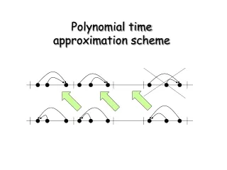
11. Pruning Candidates (3) (b) (a) Both (a) and (b) look the same to the source. Remove the one with the worse slack and cost (4) 11

12. Merging Branches Left Candidates Right Candidates O(n1n2) solutions after each branch merge. Worst-case O((n/m)m) solutions. 12

13. inferior/dominated if C1 C2,W1 W2 and Q1 Q2 DP Properties (Q1,C1,W1) • Non-dominated solutions are maintained - for the same Q and W, pick min C • # solutions depends on # of distinct W and Q, but not their values (Q2,C2,W2)

14. Gap 1990 1991 ……. 1996 ……. 2003 2004 ……. 2008 2009 Previous Works van Ginneken’s algorithm Chen and Zhou’s algorithm Shi and Li’s algorithm NP-hardness proof Lillis’ algorithm

15. Bridging The Gap • A Fully Polynomial Time Approximation Scheme (FPTAS) • Provably good • Within (1+ɛ) optimal cost for any ɛ>0 • Runs in time polynomial in n (nodes), b (buffer types) and 1/ɛ • Best solution for an NP-hard problem in theory • Highly practical We are bridging the gap! 15

16. The Rough Picture W*: the cost of optimal solution Key 1: Efficient checking Key 2: Smart guess Make guess on W* Not Good Check it Good (close to W*) Return the solution 16

17. Key 1: Efficient Checking Benefit of guess • Only maintain the solutions with cost no greater than the guessed cost • Accelerate DP

18. The Oracle Setup upper and lower bounds of cost W* Guess x within the bounds Update the bounds Oracle (x) • Oracle (x): the checker, able to decide whether x>W* or not • Without knowing W* • Answer efficiently 18

19. Construction of Oracle(x) Scale and round each buffer cost Dynamic Programming Only interested in whether there is a solution with cost up to x satisfying timing constraint Perform DP to scaled problem with n/ɛ. Runtime polynomial in n/ɛ 19

20. Scaling and Rounding • Rounding error at each buffer xɛ/n, total rounding error xɛ. • Larger x: larger error, fewer distinct costs and faster • Smaller x: smaller error, more distinct costs and slower • Rounding is the reason of acceleration buffer costs are integers due to rounding and are bounded by n/ɛ. Buffer cost xɛ/n 2xɛ/n 3xɛ/n 4xɛ/n 0

21. DP Results DP result w/ all w are integers  n/ɛ • Yes, there is a solution satisfying timing constraint • No, no such solution • With cost rounding back, the solution has cost at most n/ɛ • xɛ/n + xɛ= (1+ɛ)x > W* • With cost rounding back, the solution has cost at least n/ɛ • xɛ/n = x  W*

22. Rounding on Q • # solutions bounded by # distinct W and Q • # W = O(n/ɛ1) • Rounding before DP • # Q • Round up Q to nearest value in {0, ɛ2T/m , 2ɛ2T/m, 3ɛ2T/m,…,T }, in branch merge (m is # sinks) • Rounding during DP • # Q = O(m/ɛ2) • # non-dominated solutions is O(mn/ɛ1ɛ2) 0 ɛ2T/m 2ɛ2T/m 3ɛ2T/m 4ɛ2T/m

23. Q-W Rounding Before Branch Merge Q T 4ɛ2T/m 3ɛ2T/m 2ɛ2T/m ɛ2T/m W 0 1 2 3 4 n/ɛ1

24. Solution Propagation: Add Wire • c2 = c1 + cx • q2 = q1 - (rcx2/2 + rxc1) • r: wire resistance per unit length • c: wire capacitance per unit length x (v1, c1, w1, q1) (v2, c2, w2, q2)

25. Solution Propagation: Insert Buffer (v1, c1, w1, q1) (v1, c1b, w1b, q1b) • q1b = q1 - d(b) • c1b = C(b) • w1b = w1 + w(b) • d(b): buffer delay

26. Buffer Insertion Runtime

27. Solution Propagation: Merge • Round q in both branches • cmerge = cl + cr • wmerge = wl + wr • qmerge = min(ql , qr) (v, cl , wl , ql) (v, cr ,wlr,qr)

28. Branch Merge Runtime - 1 Target Q=0

29. Branch Merge Runtime - 2 Target Q= ɛ2T/m

30. Branch Merge Runtime -3 Target Q= 2ɛ2T/m

31. Branch Merge Runtime -4

32. Timing-Cost Approximate DP • Lemma: a buffering solution with cost at most (1+ɛ1)W* and with timing at most (1+ɛ2)T can be computed in time

33. Key 2: Geometric Sequence Based Guess • U (L): upper (lower) bound on W* • Naive binary search style approach • Runtime (# iterations) depends on the initial bounds U and L Set U and L on W* x=(U+L)/2 Oracle (x) W*<(1+ɛ)x W*  x U= (1+ɛ)x L= x

34. Adapt ɛ1 • Rounding factor xɛ1/n for W • Larger ɛ1: faster with rough estimation • Smaller ɛ1: slower with accurate estimation • Adapt ɛ1 according to U and L

35. U/L Related Scale and Round Buffer cost 0 U/L xɛ/n xɛ/n

36. Conceptually • Begin with large ɛ1 and progressively reduce it (towards ɛ) according to U/L as x approaches W* • Fix ɛ2=ɛ in rounding Q for limiting timing violation • Set ɛ1 as a geometric sequence of …, 8, 4, 2, 1, 1/2, …, ɛ • One run of DP takes about O(n/ɛ1) time. Total runtime is bounded by the last run as O(… + n/8 + n/4 + n/2 + … + n/ɛ) = O(n/ɛ), independent of # iterations

37. Oracle Query Till U/L<2 37

38. Mathematically

39. The Algorithmic Flow Set U and L of W* Adapting ɛ1 =[U/L-1]1/2 Update U or L Set x=[UL/(1+ ɛ1)]1/2 Oracle (x) U/L<2 Compute final solution

40. When U/L<2 Scale and round each cost by Lɛ/n • At least one feasible solution, otherwise no solution with cost 2n/ɛ • Lɛ/n = 2L  U • A single DP runtime W=2n/ɛ Run DP Pick min cost solution satisfying timing at driver 40

41. Main Theorem • Theorem: a (1+ ɛ) approximation to the timing constrained minimum cost buffering problem can be computed in O(m2n2b/ɛ3+ n3b2/ɛ) time for 0<ɛ<1 and in O(m2n2b/ɛ+mn2b+n3b) time for ɛ1

42. Experiments • Experimental Setup • 1000 industrial nets • 48 buffer types including non-inverting buffers and inverting buffers • Compared to Dynamic Programming

43. Cost Ratio Compared to DP Buffer Cost Ratio 43 Approximation Ratio ɛ

44. Speedup Compared to DP Speedup 44 Approximation Ratio ɛ

45. Timing Violations (% nets) Timing violations Approximation Ratio ɛ

46. Cost Ratio w/ Timing Recovery Buffer Cost Ratio 46 Approximation Ratio ɛ

47. Speedup w/ Timing Recovery Speedup 47 Approximation Ratio ɛ

48. Observations • Without timing recovery • FPTAS always achieves the theoretical guarantee • Larger ɛ leads to more speedup • On average about 5x faster than dynamic programming • Can run 4.6x faster with 0.57% solution degradation • <5% nets with timing violations • With timing recovery • FPTAS well approximates the optimal solutions • Can still have >4x speedup

49. NP-Hardness Complexity Exponential Time Algorithm Our Bridge

50. Conclusion • Propose a (1+ ɛ) approximation for timing constrained minimum cost buffering for any ɛ > 0 • Runs in O(m2n2b/ɛ3+ n3b2/ɛ) time • Timing-cost approximate dynamic programming • Double-ɛ geometric sequence based oracle search • 5x speedup in experiments • Few percent additional buffers as guaranteed theoretically • The first provably good approximation algorithm on this problem