The POPULUS modelling software

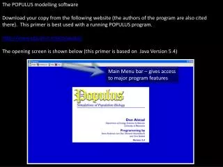
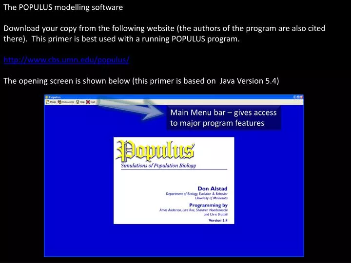
1. The POPULUS modelling software Download your copy from the following website (the authors of the program are also cited there). This primer is best used with a running POPULUS program. http://www.cbs.umn.edu/populus/ The opening screen is shown below (this primer is based on Java Version 5.4) Main Menu bar – gives access to major program features

2. The POPULUS modelling software Depending on your screen size, you may need to adjust the POPULUS program windows. Each of them can be scaled by clicking-and-dragging on any edge (just like any other window). POPULUS windows may be repositioned by clicking-and-dragging on their heading. POPULUS windows may be scaled by clicking-and-dragging on any edge.

3. The POPULUS modelling software A Help document can be accessed by clicking on the Help button in the menu bar. The help document is a pdf file and will require a pdf reader.

4. The POPULUS modelling software Access the models by clicking on the Model button. We’ll discuss Density-Dependent growth in this section. • NOTE: This primer assumes that you have mastered the lesson(s) on: • Density-Independent growth models

5. The POPULUS modelling software: Density-Dependent Growth This refers to the starting population size you wish to define (we will be using the default value of 5). K is the Carrying Capacity of the environment for the species. It is a limit on population size imposed by the enviroment. This refers to the number of generations you wish the model to run. We will be using 100 throughout our simulations. (Change this setting to 100).

6. The POPULUS modelling software: Density-Dependent Growth We will use this model type throughout the simulation. This graph shows the change in population abundance over time. This a plot which represents the K as a straight line. We will use this plot when visualizing growth vectors.

7. The POPULUS modelling software: Density-Dependent Growth Input the following parameters and click on ‘View’ to see how the graph is plotted.

8. The POPULUS modelling software: Density-Dependent Growth Stationary phase – birth and death rates balance out and net growth becomes zero The value obtained when the stationary phase is projected to the y-axis is known as the K or carrying capacity. Log phase – population growth maximized (exponential) Lag phase – abundance minimal; population still adjusting

9. The POPULUS modelling software: Density-Dependent Growth Let’s see what happens when the K of a population is changed. POPULUS allows the modelling of multiple populations in one graph. This is done by clicking the A to D tabs shown below. Each tab will allow users to set parameters for each population. Click on the check box before moving on to another tab. Shown below is tab C. After setting the K for each population (KA = 500; KB = 300; KC = 200; KD = 100), click on view to see the graphs. These tabs give access to the parameter options for up to four populations. Click to shift from A to D. Click on this check box to activate the population. If this is left unchecked, the population growth model will not be plotted. Change the K for each population as follows KA = 500; KB = 300; KC = 200; KD = 100.

10. The POPULUS modelling software: Density-Dependent Growth You should see the graph below if you set the parameters correctly. Notice that the level of the stationary phase changes according to the set K for each population. Biologically speaking, this means that each population has a unique way of maximizing the resources available in the environment. From another perspective, the K reflects the tolerance level of the environment for the population. Populations with low K have great demands on the environment (they need huge amounts of food and water and large areas for shelter) hence their numbers are naturally low. How many elephants can HEDCen support? How many ants? Those two questions should make the concept of K very clear to you. The differences in K can be seen in the levels of the stationary phases. NOTE: There is a very real possibility of misinterpreting this graph. Remember that this shows the growth curves of 4 different populations growing separately. There is no competition here. The graphs were plotted together to aid comparative analysis only.

11. The POPULUS modelling software: Density-Dependent Growth Close the active graph and reset the K of the four populations to 500. Now let’s see the effect of changing growth rates. Set the r of each population to the following values: rA = 0.1; rB = 0.2; rC = 0.3; rD = 0.4 and click ‘View.’ The graph below should appear: The log phases of the growth curves (encircled portion) have become steeper with increasing r values (the red line is for Population A, r = 0.1 and the pink is for D, r=0.4). Biologically speaking, this means that populations with higher r are able to reach their K sooner. Think of it this way: suppose two people can finish at most 3 pizza slices each (their K = 3). Person X, however, is a fast eater while Person Y likes to chew slowly. Who do you think will be able to finish 3 slices sooner?

12. The POPULUS modelling software: Density-Dependent Growth Close the active graph and uncheck the box for populations B to D. Set the parameters of Population A according to the options below. Note the different Plot Type used (checked). This will allow us to plot growth vectors. Click ‘View’. 

13. The POPULUS modelling software: Density-Dependent Growth The diagonal line represents the K of the population. The area below the line is the area of growth for the population (it has net yet maximized the environment; it has not yet reached its K). The growth vector for the population therefor points to the right (towards positive infinity of the x-axis). The area above the diagonal is the “Kill Zone”. The population has grown beyond its K, hence it starts to decline (there is not enough food or shelter for everyone). Thus the growth vector points to the left. These growth vectors are used for the next model- Competition. The diagonal represents the K of the population. It is also known as the ZNGI or the Zero Net Growth Isocline. Recall that the K is the limit the environment imposes on the population. Once it has reached its K (its ZNGI), it will not grow anymore. End of primer. Press any keyboard button to exit.