so the mean pressure will be

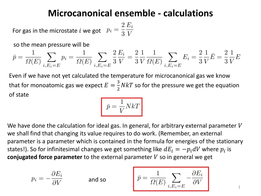
1. Microcanonical ensemble - calculations For gas in the microstate we got so the mean pressure will be Even if we have not yet calculated the temperature for microcanonical gas we know that for monoatomic gas we expect so for the pressure we get the equation of state We have done the calculation for ideal gas. In general, for arbitrary external parameter we shall find that changing its value requires to do work. (Remember, an external parameter is a parameter which is contained in the formula for energies of the stationary states!). So for infinitesimal changes we get something like where is conjugated force parameter to the external parameter so in general we get and so

2. Microcanonical ensemble - temperature We said that we calculate the macroscopic quantities expected in equilibrium macrostate as mean values of the microstate values of the corresponding physical quantities over the microcanonical ensemble. However there are physical quantities which are well defined only for macrostates, they have no analog for microstates. These are for example entropy, temperature and chemical potential. This is not obvious especially for temperature: one might try to define temperature for example for an isolated gas microstate as the total energy divided by the number of molecules (perhaps adding some factors like ). But this is just expressing energy in units of Kelvin. This does not respect the definition of temperature by the zeroth law of thermodynamics: its role of the quantity controlling the mutual equilibrium. Equilibrium state is a property of macrostate. So we have to calculate temperature of a microcanonical ensemble system using a thermodynamic definition like • first calculate the entropy as • then calculate the temperature as Technically, however, it is almost impossible to calculate entropy using the above formula, we shall calculate the entropy of gas later using technology of grandcanonical ensemble.

3. Canonical ensemble We shall now consider a system whose temperature is kept constant by a thermostat (“dwarf boiler attendant”). To make the theoretical analysis easier, we shall not consider real technologic thermostat but an abstract model: our system in thermal contact with a very large system called reservoir. Energy exchange through the thermal contact are negligible for the extremely large reservoir. So we can consider the temperature of the reservoir as constant and given. So we have a theoretically analyzable model of thermostat. System of our interest will be called just “system”, it is in thermal contact with a large “reservoir”. The system and the reservoir together form “supersystem”. The supersystem can be considered as isolated, the total energy of the supersystem is considered to be fixed, so we can represent the supersystem by a microcanonical ensemble. The energy of the system will be denoted as , of the reservoir as and of the supersystem as . The microstate of the supersystem is composed by the state of the system and by the state of the reservoir . So the supersystem state is a pair .

4. Canonical ensemble The supersystem microstate is a pair (𝒊,𝑰). Now suppose, that we are interested in a quantity, which is defined for the system alone. That is its value depends only on the system state and not on the reservoir state . Still, we can calculate its mean value using a the microcanonical ensemble for the whole supersystem: Do notice, that the value does not have the index , since the value of does not depend on the reservoir state . Still, in the formula above, we have to sum over all the values of the index . This means, that the terms in the sum above having the same index but different values of contribute to the sum by a same value. So we can group the terms to groups having the same value of and express the mean value as Here is the number of states of the reservoir such that combined with the system state they have the right total energy . So it is the number of terms in the original sum containing the system state . So the rewritten sum is correct.

5. Canonical ensemble Now we rewrite through the entropy and get Since the reservoir is much larger than the system and we expand the function in the exponent to the first order in Taylor series: Using the formula we get The factor in front of the sum “does not feel” the system at all neither it feels what quantity we are interested in, it is just a constant. It is in fact a normalization constant.

6. Canonical ensemble So what have we got? In the formula is the temperature of the reservoir but because of the equilibrium through the thermal contact it is also the temperature of the system. So we can calculate any mean value concerning the system by forgetting about the reservoir: there is no more any mentioning of the reservoir in the above formula. The formula looks like a standard formula for calculating the mean values if we interpret the factor as a probability of the system microstate . So the rule: The ensemble representing a macrostate of a system with a given temperature (kept constant by a suitable thermostat) can be constructed taking all the possible microstates (with arbitrary energy, but fixed number of particles ), each with the probability such an ensemble is called canonical ensemble.

7. Canonical ensemble – comments • Deriving canonical distribution from the microcanonical we did a “forbidden operation”: We have exponentiate the entropy. This is dangerous, since is “fuzzy defined” what makes no problems after taking logarithm of it what gives entropy. We have already warned that exponentiating back the entropy returns which again is “fuzzy” but we have no control on it. So maybe the effective probabilities of the system states are not correct !? The point is that we are not interested in probabilities, we want to calculate mean values: summing over probabilities. And the states with debatable probabilities are anyhow those with marginal probabilities which do not contribute to the sums significantly. The problem might be only with normalization, but we have to recalculate normalization anyhow (see next slides) and that will be done with probabilities already fixed. • We expanded the entropy in the exponent only to the first order in . Could we get “a more precise” canonical distribution doing the expansion to the second order. Actually not. The reservoir is very big: you can check that the second order would be negligible. You can investigate it for some model of reservoir like ideal gas and find that the correction in the exponent would be proportional to and therefore negligible Now we rewrite through the entropy

8. Canonical ensemble – Statistical sum The normalization constant can be calculated from the condition From there we get where is sometimes called the statistical sum and it is the first thing one has to calculate when one wants to use the canonical ensemble. We have explicitly written the condition that the sum is taken only over the states with fixed . Usually one writes just and the condition is understood implicitly. A short summary of the canonical ensemble usage: • canonical ensemble is to be used when the given quantities for the system are temperature and volume (or external parameter) • the first step is to calculate the statistical sum • then the mean value of any quantity is calculated as

9. Canonical ensemble – mean values In particular the mean energy of a canonical system is given as The mean pressure (more generally the man value of the canonical force quantity conjugated to the external parameter is given as

10. Canonical ensemble – small system Deriving the canonical ensemble probabilities we have used an auxiliary large system, the reservoir, playing the role of thermostat. Inspecting the derivation we can see, that using the statistical methods and calculating the means we used the fact that the reservoir and therefore also the supersystem was large macroscopic system. We in fact did not need the system to be macroscopic. Therefore the canonical ensemble can be used also for small systems in contact with reservoir or thermostat. Even for such a small system as one particle. Let us consider gas of classical (non quantum) particles. In that case we can define a particular particle as the system of interest. (For quantum indistinguishing particles we cannot limit attention to one specific particle!) The chosen particle collides with many other particles of the gas, so we can say our particle is in thermal contact with the rest of the gas which would play the role of the reservoir (or thermostat). So we can use the technique of canonical ensemble for a small system containing just one particle. This, however, requires classical (non-quantum) statistical physics, that is classical analogue of our quantum formula which uses discrete quantum states. We shall write the relevant classical formula just intuitively, without deep discussion on the relation between quantum and classical statistics. Actually, we have already seen the Maxwell velocity distribution, so we just will point at the canonical ensemble interpretation of the Maxwell distribution

11. Canonical ensemble – Maxwell distribution We shall consider one classical particle in contact with rest of the particles in gas as a reservoir. Let us first assume there is no external field (like gravitation). Then what concerns position the particles are uniformly distributed in the container. The microstate of a particle is then given by its velocity. So we are interested to get the probability that our selected particle has velocity . Classical velocity is a continuous variable, so we have to use the probability technology for continuous variables: probability densities. Intuitively we expect that in parallel to quantum canonical distribution the probability density for velocities will be proportional to the “Boltzmann factor” For one particle and no external field the relevant energy in the formula should be just the kinetic energy so we get We got what we expected: the Maxwell distribution. The normalization constant (analog of statistical sum) we get from the condition and get what we have already seen:

12. Canonical ensemble – Boltzmann distribution In external field the gas particle distribution is no more uniform, the microstate of the particle is given by its position and velocity. So for one classical particle we get the probability density in the space This is called the Boltzmann distribution. The normalization constant is to be obtained from the condition If we are not interested by the velocity distribution, we can integrate over velocities and get the marginal spatial probability density

13. Canonical ensemble – barometric formula Applied to homogenous gravitational field we get for the marginal probability density of the -coordinate of a particle where is the mass of the particle. Then for the gas spatial particle density at the height (number of particles per unit volume) we get where is obviously the particle density at . Since ideal gas pressure is proportional to the particle density we get for the pressure distribution in isothermal atmosphere (temperature not dependent on ) This barometric formula can be used as the bases for the construction of pressure altimeter. The altitude of a plane can be determined by comparing the pressure at unknown altitude with the pressure at the ground.

14. Canonical ensemble – classical harmonic oscillator Let us consider a single harmonic oscillator in contact with a thermostat. It is “a small system at constant temperature” so we can apply the Boltzmann distribution. Without doing “too much science” around it we shall apply it just intuitively, assuming that the probability distribution in the two dimensional space of states is The normalization constant is to be get from the condition The probability density is just a double Gaussian, so the calculation is easy and we get Having this we can easily calculate the mean energy and get Here is the summary of results for single harmonic oscillator at temperature

15. Canonical ensemble – entropy We have defined entropy for isolated system as k-times the logarithm of the number of microstates corresponding to the macrostate considered (equivalently the number of states in the corresponding microcanonical ensemble). This definition cannot be extrapolated to the system in contact with the thermal reservoir: the corresponding ensemble is the canonical ensemble which is formed by all - that is an infinite number - of microstates. We have to look for some alternative definition of entropy. The notion of entropy is conceptually relevant only for macrostates of systems with very large degrees of freedom. The canonical distribution can be used also for small systems in contact with reservoir, but we need to define entropy only for very large systems. For very large systems the macroscopic values are very sharp: the values fluctuate but typically on the level of 13-th decimal place. In particular: the energy of a large canonical system is practically constant. We are unable to observe fluctuations on the 13-th decimal place. Experimentally we cannot just by measurements distinguish a canonical system with fixed given temperature from a microcanonical system with a given fixed energy. Therefore the idea: The entropy for a canonical system can be defined in two consecutive steps • Determine the mean energy of the canonical system considered. • Imagine the same system as if an isolated system with a fixed energy what would be its entropy . This is to be called the entropy of the original canonical system.

16. Canonical ensemble – entropy The above mentioned two-step process for calculating the canonical entropy can be rewritten by a single compact formula. Its derivation is a bit tricky. Here it is. We start with the definition of the statistical sum where the summation is over the states. We can regroup the terms in this sum according to the energy of states and rewrite the sum as a sum over energies as In this sum the function is a sharply rising function of while the exponent is a sharply decreasing function of . Therefore the main contribution to the whole sum comes from the terms with . The domination of the terms around is such, that in the logarithmic precision the logarithm of the sum is given by a single term (we write just instead of as it is usual in statistical physics where most of the equations are only approximate anyhow). From there we get This formula could be used as the definition of entropy of a canonical system. But we will derive still a nicer formula.

17. Canonical ensemble – entropy We start with the formula we just got and we play more with it: see the nice trick, using The last formula is very nice and compact and it can be shown that it is very general. For example it also holds for a microcanonical system where we have so we get what is just “k times the logarithm of the number of states” as it should be.

18. General ensemble – entropy The formula for entropy we have derived for the canonical ensemble can be used as a general definition of entropy for any macroscopic state, represented by a suitable statistical ensemble. Statistical ensemble in general is a set of microstates with assigned probability . Then the man value of any physical quantity which has a well defined value for any microstate from the ensemble is defined as and the entropy of that macrostate is defined as It looks as if it was a mean value of some physical quantity (entropy?) of individual microstates. This is not true. The probability is not a state variable of an individual microstate. It cannot be calculated just from microstate-defining variables. The probability is given by the weight of the microstate in the ensemble characterizing the macrostate. So one has to know the macrostate before assigning the probabilities . Actually, many textbooks basically start the introduction to statistical physics with something like the above framed text as “the basic postulate”. The general formula for entropy which looks a priori like a miraculous guess is in fact very natural for anyone who is familiar with the theory of information, where it is called “the information entropy”. The interested reader may find more in may text on advanced statistical physics.

19. Canonical ensemble – first law of thermodynamics We start with the formula for the mean energy: Now suppose our “external dwarfs” infinitesimally change the macrostate in a general way. The corresponding ensemble will be changed, that is the probabilities of the microstates will be changed by and the energies of the microstates will also be changed in general by due to some changes of external parameters (like ). The mean energy of the macrostate will be changed by The physical interpretation of the first sum is clear: energies are changed due to the change of the external parameter , so we can write We know the first term, it is the mechanical work (extracted e.g. by the dwarf piston-pusher). So the second term must be heat (performed by the boiler attendant)

20. Canonical ensemble – first law of thermodynamics Now for a canonical system we perform an ingenious trick writing Using this in the just derived formula for heat we get The first term is 0 since The second term needs another ingenious insight: indeed: So we have got, as expected

21. Canonical ensemble – partition function We have defined the statistical sum as a “normalization constant” This evokes impression that is a constant. It is to some extent true. However, a canonical system has a given temperature and volume (external parameter) . If we evaluate for arbitrary values T, we get a function . as a function is called partition function. We shall show that this function carries a lot of useful information about the canonical system considered. Let us start with calculating the mean energy: So the information on the mean energy “is coded” in the partition function. The above formula is the instruction how to decode it. In the same way one can easily prove that even higher moments are coded in the partition function. For variance one gets