Computing with Defects

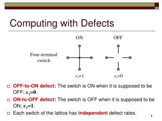
1. Computing with Defects • OFF-to-ON defect: The switch is ON when it is supposed to be OFF; x1=0. • ON-to-OFF defect: The switch is OFF when it is supposed to be ON; x1=1. • Each switch of the lattice has independent defect rates. 1 1

2. Computing with Defects • Ideally, if x1=0 then all the switches are OFF. • Ideally, if x1=1 then all the switches are ON. • We use redundancy in tolerating defects powered by percolation. 2 2

3. Percolation Theory Rich mathematical topic that forms the basis of explanations of physical phenomena such as diffusion and phase changes in materials. Broadbent & Hammersley (1957). 3

4. Percolation Theory Sharp non-linearity in global connectivity as a function of random local connectivity. 4

5. Percolation Theory p2versusp1for 1×1, 2×2, 6×6, 24×24, 120×120, and infinite size lattices. • Each square in the lattice is colored black with independent probabilityp1. • p2is the probability that a connected path exists between the top and bottom plates. 5 5

6. Margins • One-margin: Tolerable p1ranges for which we interpret p2 as logical one. • Zero-margin: Tolerable p1 ranges for which we interpret p2 as logical zero. Margins correlate with the degree of defect tolerance. 6 6

7. Implementing Boolean functions signals in: xi’s signals out: connectivity top-to-bottom / left-to-right. 7 7

8. An example with 16 Boolean inputs A path exists between top and bottom, fL = 1 8 8

9. Margin performance with a 2×2 lattice fL=x1x3+x2x4 gL=x1x2+x3x4 Different assignments of input variables to the regions of the network affect the margins. 9 9

10. One-margins (always good) ONE-MARGIN fL=0 fL=1 Defect probabilities exceeding the one-margin would likely cause an (1→0) error. 10 10

11. Good zero-margins ZERO-MARGIN fL=0 fL=1 Defect probabilities exceeding zero-margin would likely cause an (0→1) error. 11 11

12. Poor zero-margins POOR ZERO-MARGIN fL=1 fL=0 Assignments that evaluate to 0 but have diagonally adjacent assignments of blocks of 1's result in poor zero-margins 12 12

13. Lattice duality A necessary and sufficient condition for good error margins is that the Boolean functions fLand gLare dual functions. 13

14. Lattice duality fL=x1x3+x2x4 gL=x1x2+x3x4 fL ≠ gLD 14

15. Optimization problem • For a given target Boolean function fThow tooptimize of the lattice area (R×C×N×M) while meeting prescribed defect tolerances? • Determine R×C; determine N×M. 15

16. Optimization problem The Algorithm Begin with the target function fT and its dual fTD Find a lattice with the smallest number of regions that satisfies the conditions: fL = fT and gL = fTD. This determines R×C. Dependent on the defect rates of the technology, determine the required one and zero margin values. Determine the number of switches required in each region in order to meet the prescribed margins. This determines N×M.

17. Experimental Results Required lattice areas for the target functions meeting 10% one and zero margins.

18. Outline Logic synthesis for lattices of four-terminal switches. Defect tolerance for lattices of four-terminal switches. Mathematics of lattice-based computation: self-duality problem. Future Work

19. Boolean duality • Famous unsolved problem (self-duality problem): • Time complexity of testing whether a monotone Boolean function in IDNF is self-dual. Monotone: No negation IDNF: Irredundant form Self-dual:

20. Boolean duality Consider a monotone self-dual Boolean function f in IDNF with k variables and n disjuncts: Lemma (Fredman and Khachiyan, 1996; Gaur and Krishnamurti, 2008):k ≤ n2.. Theorem(Altun and Riedel, 2012):k ≤ n.

21. Number of disjuncts vs. variables Matching between a variable x and a disjunct D: There is a matching between x and D if x is a variable of D. Example: if D = x1x2 then there is a matching between x1 and D as well as x2 and D. Theorem (Altun and Riedel, 2012):Consider a monotone Boolean function f in IDNF. If f is self-dual then each variable of f can be matched with a distinct disjunct. Corollary:k ≤ n

22. Number of disjuncts vs. variables Example: Consider a monotone self-dual Boolean function • Three variables • Three disjuncts x1 x2 x2 x3 x1 x3 x1 x2 x3

23. Number of disjuncts vs. variables Example:Consider a monotone self-dual Boolean function • Six variables • Seven disjuncts x1 x2x3 x2 x3x6 x1 x3x4 x2x4x5 x1x5x6 x3x4x6 x3x5 x1 x2 x3 x4 x5 x6 k ≤ n

24. Boolean duality Self-duality problem for monotone Boolean functions with n variables and n disjuncts; k =n. Our algorithm runs in O(n4) time.

25. Self-duality problem The Algorithm Input:A monotone Boolean function f in IDNF with n variables n disjuncts. Output:If f is self-dual then “YES”; otherwise “NO”. • If f is a single variable Boolean function then return “YES”. • If f is a specific Boolean function shown below then return “YES”. • This function represents the fano plane with 7 variables and disjuncts. • If the intersection property does not hold for f then return “NO”. • If intersection property holds forfthenevery pair of disjuncts has a non-empty intersection. • If f does not have two disjuncts of size two, xaxb and xaxc then return “NO”; if it does then obtain a new function in IDNF. Repeat this step until f consists of a single variable; in this case, return “YES”.

26. Self-duality problem Example:Consider a monotone Boolean function • Seven variables and seven disjuncts; n=7. • Apply step four; xa=x1,xb=x2, andxc=x3; : • Apply step four; xa=x3,xb=x1, andxc=x4; : • Apply step four: no two disjuncts of size two. • Returns “NO”; fis not self-dual. The Algorithm If f is a single variable Boolean function then return “YES”. If f represents the Fano plane then return “YES”. If the intersection property does not hold for f then return “NO”. If f does not have two disjuncts of size two, xaxb and xaxc then return “NO”; if it does then obtain a new function in IDNF. Repeat this step until f consists of a single variable; in this case, return “YES”. 4. If f does not have two disjuncts of size two, xaxb and xaxc then return “NO”; if it does then obtain a new function in IDNF. Repeat this step until f consists of a single variable; in this case, return “YES”.

27. Outline Logic synthesis for lattices of four-terminal switches. Defect tolerance for lattices of four-terminal switches. Mathematics of lattice-based computation: self-duality problem. Future Work

28. Future work • Our model's applicability to different technologies: • Optical switch-based structures. • Arrays of single-electron transistors.

29. Future work A model with 2k terminal switches. Eight-terminal magnetic switch based array

30. Future work Correlated defect probabilities: correlated percolation.

31. Future work • Self-duality problem: • Testing whether a monotone Boolean function in IDNF is self-dual. Monotone self-duality problem for different k-n relations.