Download
1 / 31
330 likes | 603 Views
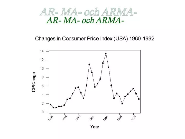
AR- MA- och ARMA-. First try: AR(1). Use MINITAB’s ARIMA-procedure. ARIMA Model ARIMA model for CPIChnge Final Estimates of Parameters Type Coef StDev T P AR 1 0,8247 0,1048 7,87 0,000 Constant 0,7634 0,3347 2,28 0,030

E N D
First try: AR(1) Use MINITAB’s ARIMA-procedure
ARIMA Model ARIMA model for CPIChnge Final Estimates of Parameters Type Coef StDev T P AR 1 0,8247 0,1048 7,87 0,000 Constant 0,7634 0,3347 2,28 0,030 Mean 4,354 1,909 Number of observations: 33 Residuals: SS = 111,236 (backforecasts excluded) MS = 3,588 DF = 31 Modified Box-Pierce (Ljung-Box) Chi-Square statistic Lag 12 24 36 48 Chi-Square 25,9 32,2 * * DF 10 22 * * P-Value 0,004 0,075 * *
ARIMA Model ARIMA model for CPIChnge Final Estimates of Parameters Type Coef StDev T P AR 1 0,8247 0,1048 7,87 0,000 Constant 0,7634 0,3347 2,28 0,030 Mean 4,354 1,909 Number of observations: 33 Residuals: SS = 111,236 (backforecasts excluded) MS = 3,588 DF = 31 Modified Box-Pierce (Ljung-Box) Chi-Square statistic Lag 12 24 36 48 Chi-Square 25,9 32,2 * * DF 10 22 * * P-Value 0,004 0,075 * *
Ljung-Box statistic: where n is the sample size d is the degree of nonseasonal differencing used to tranform original series to be stationary. Nonseasonal means taking differences at lags nearby, which can be written (1–B)d rl2(â) is the sample autocorrelation at lag l for the residuals of the estimated model. K is a number of lags covering multiples of seasonal cycles, e.g. 12, 24, 36,… for monthly data
Under the assumption of no correlation left in the residuals the Ljung-Box statistic is chi-square distributed with K – nC degrees of freedom, where nC is the number of estimated parameters in model except for the constant A low P-value for any K should be taken as evidence for correlated residuals, and thus the estimated model must be revised.
ARIMA Model ARIMA model for CPIChnge Final Estimates of Parameters Type Coef StDev T P AR 1 0,8247 0,1048 7,87 0,000 Constant 0,7634 0,3347 2,28 0,030 Mean 4,354 1,909 Number of observations: 33 Residuals: SS = 111,236 (backforecasts excluded) MS = 3,588 DF = 31 Modified Box-Pierce (Ljung-Box) Chi-Square statistic Lag 12 24 36 48 Chi-Square 25,9 32,2 * * DF 10 22 * * P-Value 0,004 0,075 * * Low P-value for K=12. Problems with residuals at nonseasonal level
PACF look not fully consistent with AR(1) More than one significant spike (2 it seems) If an AR(p)-model is correct, the ACF should decrease exponentially (montone or oscillating) and PACF should have exactly p significant spikes Try an AR(2)
ARIMA Model ARIMA model for CPIChnge Final Estimates of Parameters Type Coef StDev T P AR 1 1,1872 0,1625 7,31 0,000 AR 2 -0,4657 0,1624 -2,87 0,007 Constant 1,3270 0,2996 4,43 0,000 Mean 4,765 1,076 Number of observations: 33 Residuals: SS = 88,6206 (backforecasts excluded) MS = 2,9540 DF = 30 Modified Box-Pierce (Ljung-Box) Chi-Square statistic Lag 12 24 36 48 Chi-Square 19,8 25,4 * * DF 9 21 * * P-Value 0,019 0,231 * * OK! Still not OK
Might still be problematic. Could it be the case of an Moving Average (MA) model? MA(1): are still assumed to be uncorrelated and identically distributed with mean zero and constant variance
MA(q): • always stationary • mean= • is in effect a moving average with weights for the (unobserved) values
ARIMA Model ARIMA model for CPIChnge Final Estimates of Parameters Type Coef StDev T P MA 1 -0,9649 0,1044 -9,24 0,000 Constant 4,8018 0,5940 8,08 0,000 Mean 4,8018 0,5940 Number of observations: 33 Residuals: SS = 104,185 (backforecasts excluded) MS = 3,361 DF = 31 Modified Box-Pierce (Ljung-Box) Chi-Square statistic Lag 12 24 36 48 Chi-Square 33,8 67,6 * * DF 10 22 * * P-Value 0,000 0,000 * *
Still seems to be problems with residuals Look again at ACF and PACF of original series:
The pattern corresponds neither with AR(p), nor with MA(q) Could it be a combination of these two? Auto Regressive Moving Average (ARMA) model
ARMA(p,q): • stationarity conditions harder to define • mean value calculations more difficult • identification patterns exist, but might be complex: exponentially decreasing patterns or sinusoidal decreasing patterns in both ACF and PACF (no cutting of at a certain lag)
Always try to keep p and q small. Try an ARMA(1,1):
ARIMA Model ARIMA model for CPIChnge Unable to reduce sum of squares any further Final Estimates of Parameters Type Coef StDev T P AR 1 0,6513 0,1434 4,54 0,000 MA 1 -0,9857 0,0516 -19,11 0,000 Constant 1,5385 0,4894 3,14 0,004 Mean 4,412 1,403 Number of observations: 33 Residuals: SS = 61,8375 (backforecasts excluded) MS = 2,0613 DF = 30 Modified Box-Pierce (Ljung-Box) Chi-Square statistic Lag 12 24 36 48 Chi-Square 9,6 17,0 * * DF 9 21 * * P-Value 0,386 0,713 * *
Calculating forecasts For AR(p) models quite simple: is set to 0 for all values of k
For MA(q) ?? MA(1): If we e.g. would set and equal to 0 the forecast would constantly be . which is not desirable.
Note that Similar investigations for ARMA-models.