Download
1 / 1
10 likes | 111 Views
Bathymetry Controls on the Location of Hypoxia Facilitate Possible Real-time Hypoxic Volume Monitoring in the Chesapeake Bay. 1. Delta Modeling Associates, Inc. San Francisco, CA. 2. Virginia Institute of Marine Science Gloucester Point, VA.

E N D
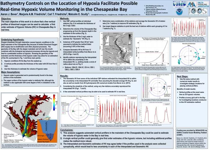
Bathymetry Controls on the Location of Hypoxia Facilitate Possible Real-time Hypoxic Volume Monitoring in the Chesapeake Bay 1. Delta Modeling Associates, Inc. San Francisco, CA. 2. Virginia Institute of Marine Science Gloucester Point, VA. 3. Woods Hole Oceanographic Institution Woods Hole, MA Aaron J. Bever1, Marjorie A.M. Friedrichs2, Carl T. Friedrichs2, Malcolm E. Scully3 : aaron@deltamodeling.com, marjy@vims.edu, cfried@vims.edu, mscully@whoi.edu Vertical Profile • Methods: • Use CBP vertical profiles at individual stations (Fig. 2) to estimate the thickness of the 2 mg/L water. • Determine the volume of the Chesapeake Bay progressing up from the deepest depth in the mainstem to the surface (Fig. 3). • Use the thickness of the 2 mg/L water to estimate the “Geometric” HV (Fig. 3). • Instances of HV greater than 20 km3 were assumed to indicate the method failed (occurring 2-18% of the time). • Compare Geometric HV to HV from 13 interpolated vertical profiles from Bever et al. (2013) (Figs. 4 and 5). • Identify stations reproducing the Interpolated HV to within the uncertainty in the Interpolated HV, i.e. plotting inside a circle of radius about one on Fig. 5: • Stations: CB4.2C, CB4.3C, CB 4.4, CB5.1, CB5.2, CB5.3, CB5.4 Objective: The main objective of this work is to show that a few vertical profiles of dissolved oxygen can be used to calculate a first order estimate of Hypoxic Volume (HV) in Chesapeake Bay in real time. DO<2 mg/L Hypoxic Thickness Determine every combination of the stations and average the Geometric HV of station sets (2 to 7 stations) to improve HV estimates (Fig. 6). Use target diagram statistics to pick the best set of stations within each grouping of 2 to 7 stations (Fig. 7). Fig. 4. Hypoxic volume interpolated from 13 CBP vertical profiles and estimated using a single station based on the Bay geometry and thickness of the 2 mg/L DO water. Missing Geometric HV were estimated to be larger than 20 km3 and removed. Uncertainty in the Interpolated HV is on the order of 2.5-7.5 km3 (Bever et al., 2013). • Underlying Hypothesis: • Oxygen drawdown through respiration causes hypoxic conditions in the deep mainstem of the Chesapeake Bay because of limited Dissolved Oxygen (DO) supply due to stratification and other physical processes. The geometry of the Bay with the deeper mainstem and sill near the mouth combines with the biological and physical processes driving the hypoxia and lead to a predictable location of hypoxia. Knowing the geometry of the mainstem and the thickness of the hypoxic water may allow for an estimation of the HV, summarized in Fig. 1 and three main points: • Hypoxic conditions fill the Bay from the seabed up. • A vertical profile provides the thickness of the water with DO less than 2 mg/L. • Use this thickness to estimate the volume of hypoxic water. • Major Assumptions: • Hypoxic water is generated and is predominantly found in the deep portion of the mainstem. • The upper surface of the hypoxic water is relatively flat, although the method is also applicable with some degree of tilt or undulation to the surface. Hypoxic Volume: ~10 km3 Thickness: 20 m Fig. 3. Volume of the mainstem Chesapeake Bay at varying heights above the deepest depth. The volume is limited to simply the mainstem and is shown to only 25 m thickness to highlight the portion of the Bay hypoxia actually occurs. Fig. 5. Target diagram comparing the Geometric HV from individual stations to that interpolated from the vertical profiles of 13 stations. The circle of radius about one equals an estimate of the uncertainty in the Interpolated HV (5 km3) due to spatial interpolation and non-synoptic sampling. Fig. 2. Chesapeake Bay bathymetry and station locations. Circles show all considered Chesapeake Bay Program station locations. Triangles identify the seven best stations for estimating the Geometric hypoxic volume. Results: The Geometric HV from seven of the individual CBP stations estimated the Interpolated HV to within the uncertainty in the Interpolated HV and better than assuming the decadal average HV (Fig. 5), and also as well as results from 3D hydrodynamic DO numerical models from Bever et al. (2013). Considering the simplicity of the method, using very few stations accurately reproduced the Interpolated HV (Figs. 7 and 8). A few automated vertical profilers may be able to be used to estimate HV in real time. • Next Steps: • Use the same method with numerical model results to investigate strategic locations for placing vertical profilers. • Benefits of model results: • Vertical profiles at the exact same time as 3D hypoxic volumes. • Profiles at every grid cell in the Bay for investigating locations conducive to this HV estimation method. Best set based on total RMSD (set shown on Fig. 7). Fig. 6. Target diagram showing how well the averaged Geometric HV from each combination of 2 stations reproduced the Interpolated HV. Number of Stations Averaged For Geometric HV Meters Fig. 7. Target diagram showing how well the best combination of stations in each set of averaged Geometric HV reproduced the Interpolated HV. Fig. 8. Hypoxic Volume interpolated from 13 CBP vertical profiles and estimated based on the geometry of the Bay and thickness of the 2 mg/L DO water using the average of the Geometric HV estimated from two stations, CB 4.4 and CB 5.3. Conclusions: This analysis suggests automated vertical profilers in the mainstem of the Chesapeake Bay could be used to estimate the volume of hypoxic water in the Bay in real time. A single vertical profiler could generally give first order estimates of the hypoxic volume, but including additional profiles makes the method more robust. The Interpolated and Geometric estimates of HV may agree better if the profiles used in the analysis were collected synoptically, which would lead to less uncertainty in each of the Interpolated and Geometric HV. Funding was provided by NOAA/IOOS via SURA’s Coastal Ocean Modeling Testbed (COMT). • Idealized surface of the 2 mg/L DO water. Bever, A.J., M.A.M. Friedrichs, C.T. Friedrichs, M.E. Scully, and L.W.J. Lanerolle. 2013. Combining observations and numerical model results to improve estimates of hypoxic volume within the Chesapeake Bay, USA. Journal of Geophysical Research, Oceans. 118. doi:10.1002/jgrc.20331 • Hypoxic Volume = Volume from seabed to 2 mg/L surface Deepest Bay Depth Fig. 1. Conceptual figure showing the 3D bathymetry of the middle and northern portion of Chesapeake Bay with a hypothetical 2 mg/L water surface (hatched layer) and conceptual cross section through the main stem showing how a vertical profile could be used to determine the thickness of the hypoxic bottom layer.