Download
1 / 16
160 likes | 232 Views
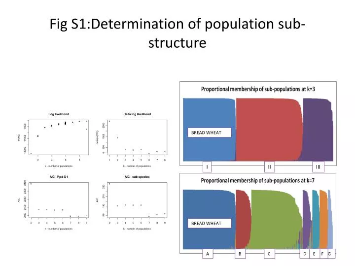
Fig S1:Determination of population sub-structure. BREAD WHEAT. I. II. III. BREAD WHEAT. A. B. C. D. E. F. G. Figure S2: Frequency based distance measures separated the bread wheat varieties from north western Europe from those originating in south eastern Europe.

E N D
Fig S1:Determination of population sub-structure BREAD WHEAT I II III BREAD WHEAT A B C D E F G
Figure S2: Frequency based distance measures separated the bread wheat varieties from north western Europe from those originating in south eastern Europe • Bread wheat is most closely related to members of sub-populations D & E (k=7), (shown in green and gold) • While bread-wheat from south eastern and north-western fall into separate clades, their D-genomes share a common (monophyletic) origin • Note: Sub populations k = 7 are designated by the following colours • Population A: Red • Population B: Pale blue • Population C: Blue • Population D: Green • Population E: Gold • Population F: Orange • Population G: Magenta Sub pops D & E Bread wheat
Figure S12: Potential evapo-transpiration among sub-populations
Figure S15: The Kullback-Leibler distances between sub-populations calculated by STRUCTURE Sub population III (at k=3) Sub population II (at k=3)
Figure S16: PCO: diversity among 232 Ae. tauschii accessions revealed by SSR data, KASPar data and both data types used in combination. Accessions belonging to Structure sub-population II are shown in red