WHY ARE DBNs SPARSE? Shaunak Chatterjee and Stuart Russell, UC Berkeley

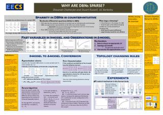
1. WHY ARE DBNs SPARSE? ShaunakChatterjee and Stuart Russell, UC Berkeley • Dynamic Bayesian Networks (DBNs) • What are DBNs? • DBNs are a flexible and effective tool for representing and reasoning about stochastic systems that evolve over time. Special cases include hidden Markov models(HMMs), factorial HMMs, hierarchical HMMs, discrete-time Kalman filters and several other families of discrete-time models. • The stochastic system’s state is represented by a set of variables Xt for each time t ≥ 0 and the DBN represents the joint distribution over the variables {X1, X2, …, X∞}. Typically, it is assumed that the system’s dynamics do not change over time, so the joint distribution is captured by a 2-TBN (2-Timeslice Bayesian Network), which is a compact graphical representation of the state prior p(X0) and the stochastic dynamics p(Xt|Xt+1). • Structured Dynamics: • The dynamics are represented in factored form via a collection • of local conditional • models • p(Xit+1|∏(Xit+1)) • where ∏(Xit+1)) are • the parent variables • of Xit+1 in slice t or t+1. • Inference in DBNs: • Exact inference is tractable for a few special cases, namely HMMs and Kalman Filter models. For general DBNs, the computational complexity for exact inference is exponential in the number of variables for a large enough time horizon (Murphy, 2002). • Approximate inference is much more popular.Boyen-Koller (BK) algorithm and Particle Filtering algorithms have been widely used. • Structure learning for DBNs has also been studied (Friedman et al, 1998). However, till date, DBNs are mostly constructed by hand. • Applications: • DBNs have been extensively used in: • Speech processing • Traffic modeling • Modeling gene expression data • Figure tracking • and in numerous other applications. Widely varying timescales: An overview Chemical Reactions: Michaelis-Menten kineticsmakes the quasi-steady-state assumption that the concentration of substrate-bound enzyme changes much more slowly than that of product or substrate. Recent works separate slow and fast timescales in the chemical master equation (CME) yielding separate reduced CMEs (see Gomez-Uribe et al) Gene Regulatory Networks: Arkin et. al. proposed an abstraction methodology using rapid equilibrium and quasi-steady-state approximations. Mathematics and Physics: Homogenization to replace rapidly oscillating coefficients. Sparsity in DBNs is counter-intuitive Consider the unrolled version of a sample DBN The longer timstep DBN becomes fully connected • How large a timestep? • Critical decision in the design of a DBN • Small enough so that fastest changing variable has a small probability of changing state • Could result in gross inefficiency! • Large timestep would be very efficient • Stochastic differential equations (SDEs) to DBNs • SDEs describe the stochastic dynamics of a system over an infinitesimally small timestep • DBNs are approximate representations of the SDEs over a finite timestep • Approximate since the exact model created by integrating the SDE over a finite timestep would result in a completely connected DBN • Most DBNs modeling real-life stochastic processes are sparse • The sparsity of these DBNs make them more tractable • They are designed by humans who make implicit approximations Marginalize out time slices t+1 and t+2 Fast variables in ∂-model and Observations in ∆-model • Body temperature (BT) and Thermometer temperature (TT) • Both variables are discretized (binary) for simplicity • Body temp. has slow dynamics compared to the thermometer • BTTT link approximated by steady state distribution • Key Questions • How to choose an appropriate ∆? • Topology of ∆-model • Any generally applicable rules? • Characterize the approximation error Bad approximation for 1-second timestep Good approximation for 60-second timestep Definitions: Timescale The timescale of a variable is the expected number of timesteps for which it stays in its current state (for a discrete state space). In a general DBN, let ∏(Xt+1) denote the parents of Xt+1 in the 2-TBN excluding Xt. Let pki,j = p(Xt+1=j|Xt=i, ∏(Xt+1)=k). Ti,kX= 1/(1- pki,i) is the timescale of X in state i when its parents are in state k. lX = mini,kTi,kX; hX = maxi,kTi,kX In a DBN with 2 variables X and Y, if lX >> hY then Y is a fast variable with respect to X. The timescale separation between X and Y is given by the ratio lX/hY. For a cluster of variables C = {X1,…,Xn}, the timescale bounds are defined by lC = minXiєClXiand hC = minXiєChXi. Larger timescale separations result in more accurate models for larger timesteps. Stationary distribution When lX>>hY the stationary distribution of Y given X=k is the limiting distribution of Y if X is “frozen” at k. This is the steady-state approximation of Y and is also referred to as the equilibrium distribution. ∂-model to ∆-model Conversion Topology changing rules • Approximation scheme: • Consider the 2-variable DBN where s is a slow variable and f is a fast variable (w.r.t. s) • ∂ denotes a short timestep and ∆ denotes a long timestep. • ∂-model Exact ∆-model Approximate ∆-model • In the approximate∆-model, • sf : stationary distribution of f for a fixed s • ^ • ss : ( P(st+1|st) )∆/∂ , where Error Characterization: If the conditional probabilities of the ∂-model have the following structure then for є<<1 and times ∆/∂ upto O(1/є), the approximation scheme for ss has an error of O(є). (Proof in paper) The error of the limiting distribution decays exponentially. Rule 1: If f1 and f2 have no cross links in ∂-model then they have no cross links in ∆-model Rule 2: If f1 and f2 have cross links in ∂-model then they are linked in ∆-model Rule 3: If s2 is a parent of f and f is parent of s1 in ∂-model then s2 is a parent of s1 in ∆-model Experiments pH control mechanism in the human body There are 4 different timescales in this DBN. Lighter shade represents slower timescale and darker shade represents faster timescale. General Algorithm: Given the exact ∂-model, the approximation scheme can be used to create a sequence of DBNs for various values of ∆, depending on the number of timescale separable clusters. For the algorithm, we assume the DBN has n variables X1, X2,…, Xn. 1. For each variable Xi, determine lXi and hXi 2. Cluster the variables in {C1, …, Cm} (m≤n) such that єi = (hCi/lCi+1) << 1, i.e. there is significant timescale separation between successive clusters 3. Repeat for i=1, 2,…, m-1 3.1. ∆i = ∆i-1 O(1/ єi) 3.2. Ci is the fast cluster and Cj (j>i) are slow clusters. Compute the stationary distribution of Ci conditioned on each configuration of its slower parents. 3.3. In the worst case, all Cj’s become fully connected in the ∆i model. If there are no links from Ci to Cj in the exact, then the {Cj}{Cj} link is exact. Accuracy of approximate models Speedup ←Fig 1. Avg. L2 error of joint belief vector Fig. 2.→ Accuracy in tracking the marginal distribution of pH