Download
1 / 35
350 likes | 537 Views
Stochastic Differential Equation Modeling and Analysis of TCP - Windowsize Behavior . Presented by Sri Hari Krishna Narayanan (Some slides taken from or based on presentations by Vishal Mishra). Outline. Introduction TCP window Algorithms

E N D
Stochastic Differential Equation Modeling and Analysis of TCP - Windowsize Behavior Presented by Sri Hari Krishna Narayanan (Some slides taken from or based on presentations by Vishal Mishra)
Outline • Introduction • TCP window Algorithms • Poisson counter driven stochastic differential equations • Expressing windowsize changes • Results • Statistical tests
Introduction • This work is directly related to Ross’ presentation last week. The authors propose a new model which is simpler and work with the same data as the previous paper to obtain similar results. • TCP is the protocol of choice for communication for many applications. • Modeling TCP is hence important. • Other applications may use other protocols • TCP friendliness • TCP shares the bandwidth fairly amongst hosts competing for network bandwidth
TCP Congestion Control: window algorithm • Window: can send W packets at a time • increase window by one per RTT if no loss, W <- W+1 each RTT • decrease window by half on detection of loss W <- W/2 slide taken from presentation by Vishal Mishra
receiver W sender TCP Congestion Control: window algorithm Window: can send W packets • increase window by one per RTT if no loss, W <- W+1 each RTT • decrease window by half on detection of loss W <- W/2 slide taken from presentation by Vishal Mishra
receiver W sender TCP Congestion Control: window algorithm • Window: can send W packets • increase window by one per RTT if no loss, W <- W+1 each RTT • decrease window by half on detection of loss W <- W/2 slide taken from presentation by Vishal Mishra
TCP loss indications at the source • There are two kinds • Time Outs(TO) • Triple Acknowledgements (TD) • Effects on the TCP windowsize • TO causes windowsize to become 1 • TD causes windowsize to halve • When there is no packet loss, the windowsize increases.
Other models • Model TCP from the point of view of the source • Packets that the source injects into the network . • Each packet has an associated loss probability. p • Identical for each packet • Can be dependent on factors such as the current windowsize
This model • Models losses in a network centric way • The network is the source of the congestion • Not the packets? • Losses are events that arrive at the source • Arrivals are then modeled using statistical analysis • In this case arrivals are modeled as a Poisson process.
Loss Indications arrival rate l Traditional, Source centric loss model New, Network centric loss model Sender Sender Loss Probability pi Loss model enabled casting of TCP behavior as a Stochastic Differential Equation, roughly SDE based model slide taken from presentation by Vishal Mishra
Networkis a (blackbox) source of R and l R l l Solution: Express R and l as functions of W (and N, number of flows) R Network Refinement of SDE model Window Size is a function of loss rate (l) and round trip time (R) W(t) = f(l,R) slide taken from presentation by Vishal Mishra
Poisson Process • What is it? • Process with exponential arrival times • Arrivals are independent of each other • Can be used to model natural occurrences • Spotting fish in the ocean • Occurrence of soft errors
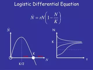
Traffic model • The increase in windowsize • Rises by 1 for every round trip time (RTT) • Instead of step increase, the increase is considered to be continuous and represented as dt/RTT • Falls by half for TD • Falls to 1 for a TO
Poisson counter • Poisson process N with arrival rate • dN ={ 1 at Poisson arrival { 0 elsewhere E[dN] = dt This basically means that for poisson loss events in time dt, there will be spikes.
Poisson Counter Driven Stochastic differential equations (SDE) • Dx = f(x(t))dt+∑gi(x(t))dNi • dW = (dt /RTT) + (-W/2)dNTD +(1-W)dNTO • First term indicates the additive increase of the TCP window • Second and Third represent the multiplicative decrease.
1/RTT W (-W/2)dNTD +(1-W)dNTO SDE Graphical Representation Changing Window size Time
What to do with the SDE • There is a lot of mathematics possible • This mathematics evaluates the expected value of the windowsize and the throughput of the network at steady state. • E[W] =(1/RTT + TO) /(TD /2 + TO ) • R =(1/RTT)*E[W] =(1/RTT)(1/RTT + TO) /(TD /2 + TO )
1/RTT W (-W/2)dNTD +(1-W)dNTO Windowsize at steady state Changing Window size Time
Maximum windowsize considerations • Restricts the maximum value of the windowsize to M. • E[W] =((1- P[W=M]) /RTT + TO) /(TD /2 + TO ) • What does this mean • The continuous function rises as long as its value is not M. • In that case it remains constant. • After some mathematics, • P[W=M] =(2TO2 + TO + TO TD + TO /RTT +2/ RTT2 +2 /RTT ) (1/RTT+1)(2M TO + MTD +2 /RTT )
1/RTT M W (-W/2)dNTD +(1-W)dNTO Windowsize at steady state with maximum window size Changing Window size Time
Other TCP features • Slowstart • Considered unimportant by authors • Timeout backoff • Modeled similarly to the maximum window
Comparison with other models • This model can be transformed into one involving packet loss • Loss/sec = TO + TD • Packets/sec = R • Loss/packet = (Loss/sec) / (Packets/sec) = (TO + TD )/R
Comparison with other models • This model can be transformed into one involving no timeouts • TO = 0, no arrival of timeouts • Earlier computation of E[W] changes • P[W=M] =(2TO2 + TO + TO TD + TO /RTT +2/ RTT2 +2 /RTT ) (1/RTT+1)(2M TO + MTD +2 /RTT ) • P[W=M] = (2/ RTT2 +2 /RTT ) (1/RTT+1)(MTD +2 /RTT ) = (2/ RTT) (MTD +2 /RTT ) • Similar changes can be made to account for no maximum window size
Results -Analysis • Closely mirrors earlier work • Except at low thoughput • This represente very high loss zone (60-80%) • Does not really matter • Does not consider 1 hour traces at all • So why use this model at all? • Simpler mathematics and analysis • So how do we get this simple analytical model?
Trace analysis Loss inter arrival events tested for • Independence • Lewis and Robinson test for renewal hypothesis • A sequence of recurrences T1,T2,... is a renewal process if the time between recurrences τj = Tj −j−, j =1, 2,... (T0 = 0) are independent and identically distributed. * • Exponentiality • Anderson-Darling test • The Anderson-Darling test is used to test if a sample of data came from a population with a specific distribution….. The Anderson-Darling test is an alternative to the chi-square and Kolmogorov-Smirnov goodness-of-fit tests.** *www.public.iastate.edu/~wqmeeker/ stat533stuff/psnups/chapter16_psnup.pdf slide based on presentation by Vishal Mishra **http://www.itl.nist.gov/div898/handbook/eda/section3/eda35e.htm
Scatter plot of statistic slide based on presentation by Vishal Mishra
Experiment 1 slide taken from presentation by Vishal Mishra
Experiment 2 slide taken from presentation by Vishal Mishra
Experiment 3 slide taken from presentation by Vishal Mishra
Experiment 4 slide taken from presentation by Vishal Mishra
So are there any more magic fits and tests? • Definitely there are more traces that can fit Poisson distribution. • Motivating Example • Soft errors • Cosmic particles hit the chip to cause bit flips • The existence of these particles can be modeled using a Poisson process. • What about other distributions? • Definitely, there may be other distributions and related mathematics.