Download
1 / 31
360 likes | 522 Views
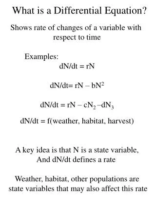
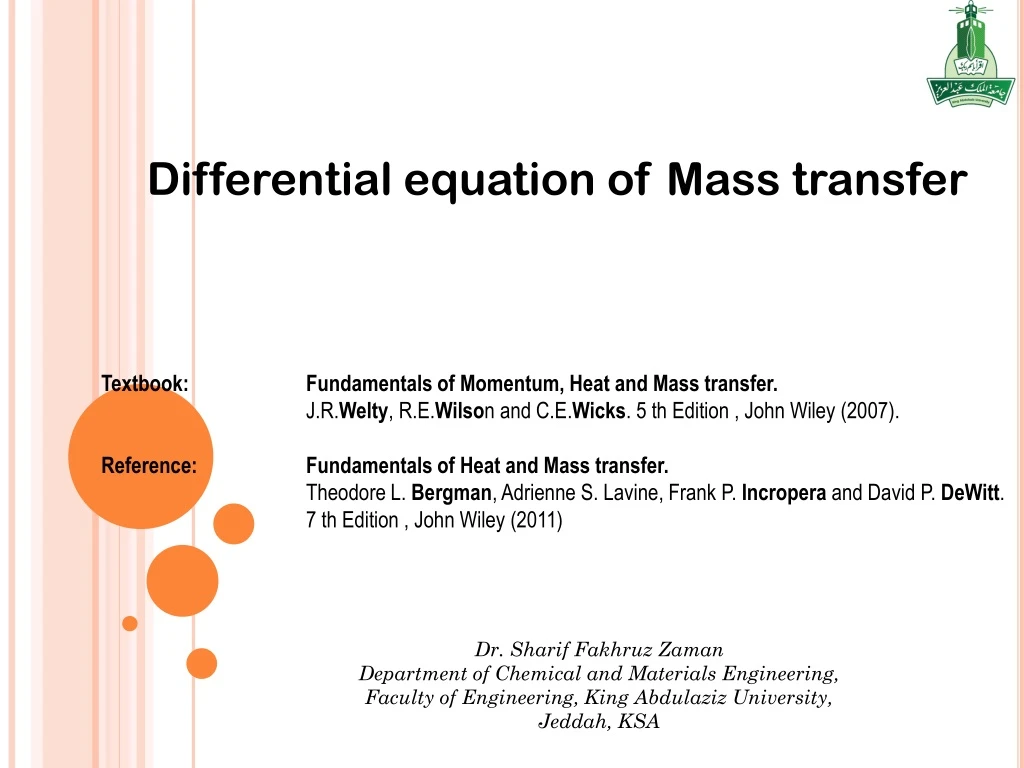
Differential equation of Mass transfer Textbook: Fundamentals of Momentum, Heat and Mass transfer. J.R. Welty , R.E. Wilso n and C.E. Wicks . 5 th Edition , John Wiley (2007). Reference: Fundamentals of Heat and Mass transfer .

E N D
Differential equation of Mass transfer Textbook: Fundamentals of Momentum, Heat and Mass transfer. J.R.Welty, R.E.Wilsonand C.E.Wicks. 5 th Edition , John Wiley (2007). Reference: Fundamentals of Heat and Mass transfer. Theodore L. Bergman, Adrienne S. Lavine, Frank P. Incropera and David P. DeWitt. 7 thEdition , John Wiley (2011) Dr. Sharif FakhruzZaman Department of Chemical and Materials Engineering, Faculty of Engineering, King Abdulaziz University, Jeddah, KSA
Chapter 25 Differential equation of Mass Transfer Example 1,2,3 Practice exercise : 3,4, 7, 8, 10,11, 13,14,15 HOME WORK : 6, 8, 11, 12. 1) Differential equation for Mass transfer (continuity equation for the mixture – what is mass efflux?) 2) special form of differential mass transfer equation (derivation of Fick's 2nd law, Fick's 2nd law for rectangular, cylindrical and spherical coordinate .. application of these equations will be in Chapter 26 to 28) 3) Commonly Encountered Boundary conditions:: ##The concentration of the transferring species A at the boundary surface is specified. How to measure different concentration ( partial pressure, mole fraction etc)? ## A reacting surface boundary is specified ## The flux of the transferring species is zero at a boundary or a at centerline of symmetry ## Convective mass transfer flux at the boundary 4) Steps for modeling process involving molecular diffusion
Differential Equations • Conservation of mass in a control volume: • Or, Out – in + accumulation – reaction = 0
Y+ΔY Δy Z+ΔZ Δy Δz (x,y,z) X+ΔX Δz Area normal to the flow in x direction : ΔYΔZ Area normal to the flow in Y direction : ΔX ΔZ Area normal to the flow in z direction : ΔX ΔY Δx Volume of the differential element : ΔX ΔY ΔZ Molar Flux (NA) =Molar rate (WA)/cross sectional area (A) Molar Rate = flow of moles of species ‘A’ per unit time Reaction rate (RA) = change of moles of species A per unit time per unit volume There are other definitions of reaction rate, i.e. per unit surface area etc.
For mass rate [out – in], • in x-dir, • in y-dir, • in z-dir, • For accumulation,
For reaction at rate rA, in – out + accumulation – reaction = 0 • Summing the terms and divide by DxDyDz, • with control volume approaching 0,
We have the continuity equation for component A, written as general form: • For binary system, • But • and
So by conservation of mass, • Written as substantial derivative, • For species A, • In molar terms, • For the binary mixture, • And for Stoichiometric reaction,
Special forms of differential mass transfer equation Application : generating concentration profile of a species, we replace the fluxes nA or NA in continuity equation with appropriate expression developed in chapter 24. Molar flux wrt fixed coordinate in space Mass flux wrt fixed coordinate in space
These two equation can be used to describe the concentration profiles within • a diffusing system. • Generalized equation. • Can be simplified by making restrictive assumptions.
Assumption 1 # (i) The density ρand diffusivity DAB are constant Dividing by the molecular wt. (MA) and rearranging
Assumption 2 # (ii) If there is no production term , no reaction, RA = 0 Thermal diffusivity Analogous to heat transfer by conduction
Assumption 3 # (iii) No fluid motion , v = 0, No production term, RA = 0, and No variation in the diffusivity or density This is known as Fick’s 2nd law of diffusion • Application of this equation is limited to ( due to the assumptions) • Diffusion in solids • Stationary liquids • Binary system of gases or liquids where NA = - NB ; • i.e. equimolar counter diffusion Analogous to Fourier’s second law of heat conduction
Assumption #4 : Further simplification # steady state assumption (iv) Steady state process, no variation of conc. or density with time - Constant diffusivity & Constant density - Constant diffusivity & Constant density & No chemical reaction - Constant diffusivity & Constant density & No chemical reaction and V =0 Laplace equation in terms of Molar concentration
Boundary conditions in mass transfer TYPE # I Concentration of transferring ( diffusing) species A at a boundary surface is specified. Example : Species ‘A’ is transferring from point 1 to point 2 in species B. Unidirectional. Consider in z direction only. The concentration of species A at point 1 ( CA1) and point 2 (CA2) is known CA1 at z1 CA2 at z2 Concentration at a surface can be expressed in different units ( denoted by subscript s) <1> Molar concentration CAs, moles of A/m3 <2> Mass concentration, ρAs, mass of A / m3. <3> Mole fraction , xAs (liquid), yAs (gas)
Case # I : when the boundary surface is defined by a pure component in one phase ( liquid phase of species A, liquid acetone, etc.) a mixture in the second phase (acetone + air mix in gas phase) • Concentration of transferring species A in the mixture at the GAS-LIQUID interface is at THERMODYNAMIC equilibrium. • >Gas mix + Volatile component A(Liquid phase) • >Gas mixture + pure volatile solid A (Air + CO2 + CO2 solid) • At the INTERFACE the partial pressure (pA) of species A is given by the • saturation vapor pressure , PAV*(get it from vapor pressure table, Antoine equation) of species A. • For liquid mixture in contract with a pure solid, (Sugar in water, NaCl salt in water etc). The concentration of species A in the liquid at the solid surface is given by the solubility limit of A in the liquid, CA*.
# For a volatile component A in gas phase in contact with a liquid phase : At the GAS-Liquid interface : for an ideal liquid system mixture : the boundary condition is given by RAOULT’S LAW PAS = Partial pressure of species A in Gas phase. xA = mole fraction in liquid phase. PA = Vapor pressure of the species A evaluated at the liquid temperature. # Species A is weakly soluble in liquid :- @ GAS LIQUID interface boundary Relation is given by Henry’s law HA = Henry’s law constant reported in Table 25.1; Unit in pressure unit; i.e. bar. xA= mole fraction in liquid phase. PA = Partial pressure of species A in GAS phase.
Boundary condition at the GAS-SOLID interface CA = Molar concentration with in the solid at interface, Kg-mol/m3. S = solubility constant, Kg-mol/m3-Pa PA = Partial pressure of A in GAS phase, Pa. Example (Solid CO2 – AIR system) Solubility constants are reported in Table 25.2.
TYPE # 2 A reaction surface boundary is specified. Three common situation {#mostly encountered in heterogeneous catalysis surface reaction.} CASE #1 : The flux of one species is related to flux of another species by chemical reaction stoichemistry. Chemical reaction at the boundary surface A + 2B 3C Relation between flux : NA = NB/2= -Nc/3 CASE # 2 : A finite rate of reaction might exist at the surface if the component A is consumed by a 1st order reaction on the catalyst surface. At Z=0. Positive Z direction is only the direction of A along Z. NA,Z |Z=0 = -Ks.CAS Ks = surface reaction rate constant, m/s. {As reaction rate is expressed in flux, actual unit for Ks for 1st order reaction =1/s}
Case # III The reaction may be so rapid at the surface that species A is a limiting reagent in the chemical reaction. CAS = 0 at the catalyst surface. CO2 O2 [B] [A] Coke [C] TYPE # III The flux of the transferring species is ZERO at the boundary surface or at the centerline of the symmetry. - Impermeable boundary - Centerline of the symmetry of the control volume (center of a sphere) the net flux is zero.
Rectangular coordinate The diffusing species cannot penetrate the boundary at z = 0 z = 0 Spherical coordinate : r= R At the center the concentration of species is same all around it. r=0 Location of the boundary is z = 0, or r = 0 .
Type # IV The convective mass transfer flux across the fluid boundary is specified. When the fluid flows over a surface the mass transfer flux can be defined by convection. At some surface located at z=0, the convective mass transfer flux across the fluid boundary Layer, CA∞ = bulk concentration of A in the flowing fluid. CAS = Surface concentration of A at z=0. Kc= convective mass transfer co-efficient.
Steps for modeling processes involving molecular diffusion • Step # 1 • Draw the picture of the physical system. • Label the important features including system boundaries. • Decide where the source and sink of mass transfer are located. • Step # 2 • Make a list of assumptions based on the consideration of the physical system • Make list of nomenclature. • Step # 3 • Pick the coordinate system , rectangular, spherical or cylindrical. • Formulate the differential material balance to describe the mass transfer • with the volume element. • Use Fick’s law or general mass transfer differential equation for mass transfer
How to simplify the general differential equation for mass transfer • Reduce or eliminate the terms that do not apply to the physical system • Steady state process , then • No chemical reaction, RA = 0 • Diffusion is one directional – i.e. in z direction Rectangular Cylindrical Spherical Or Perform shell balance for the component of interest on a differential volume element.
Simplification of Fick’s law: Establish the relationship between fluxes in the bulk contribution term. Binary mixture of A and B one dimensional flux Bulk contribution term NA = -NB , that makes yA(NA+NB) = 0 If we have yA(NA+NB) ≠ 0. NA = CAVz. And reduces to cAvz for low concentration of A in the mixture
If a differential equation for the concentration profile is desired >> Simplified form of Fick’s law must be substituted into the general differential equation of mass transfer.
Step # 4 Recognize the specific boundary condition Known concentration of species A at a surface or interface at z=0, e.g. cA =cA0 . This concentration can be specified or known by equilibrium relation. (b) Symmetry condition at a centerline of the control volume for diffusion. or no net diffusion flux of species A at a surface or interface at z = 0 , NAz|z= 0 = dcA/dz. (c) Conventive flux of species A at a surface or interface. NA = Kc(cAS – cA∞). (d) Known flux of species A at a surface or interface, at Z=0 , NAZ|Z=0 =NA0. (e) Known chemical reaction at the surface or interface. * For the rapid disappearance of species A at the surface or interface at z =0 , cAS =0. * For slower chemical reaction at the surface or interface with finite CAS, at z = 0 , NAZ = K’CAS. >> k’ = first order chemical reaction rate constant.
Step # 5 Solve the differential equation for ---- Concentration profile Mass/molar flux Mass/molar rate Mass transfer coefficient (kc) Mass transfer area Mass transfer time Etc. review your ODE and calculus course FINIS of Chapter 25