Download
1 / 37
370 likes | 379 Views
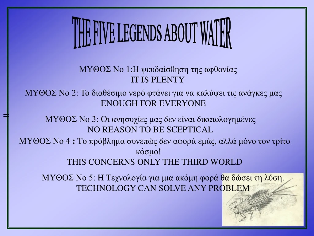
THE FIVE LEGENDS ABOUT WATER. MYΘOΣ Nο 1:H ψευδαίσθηση της αφθονίας IT IS PLENTY. MYΘOΣ Nο 2: Το διαθέσιμο νερό φτάνει για να καλύψει τις ανάγκες μας ENOUGH FOR EVERYONE. =. MYΘOΣ Nο 3: Οι ανησυχίες μας δεν είναι δικαιολογημένες NO REASON TO BE SCEPTICAL.

E N D
THE FIVE LEGENDS ABOUT WATER MYΘOΣ Nο 1:H ψευδαίσθηση της αφθονίας IT IS PLENTY MYΘOΣ Nο 2: Το διαθέσιμο νερό φτάνει για να καλύψει τις ανάγκες μας ENOUGH FOR EVERYONE = MYΘOΣ Nο 3: Οι ανησυχίες μας δεν είναι δικαιολογημένες NO REASON TO BE SCEPTICAL MYΘOΣ Nο 4:Tο πρόβλημα συνεπώς δεν αφορά εμάς, αλλά μόνο τον τρίτο κόσμο! THIS CONCERNS ONLY THE THIRD WORLD MYΘOΣ Nο 5:H Tεχνολογία για μια ακόμη φορά θα δώσει τη λύση. TECHNOLOGY CAN SOLVE ANY PROBLEM
In the near future 4 million people will suffer from water lack, even if each we spend only 40l/day/person Population increase High biotic level Overconsumption Pollution Climate change
A substance which is present at concentrations which cause harm or exceed an environmental standard is considered to pollute the environment. In disturbances reality any change or in the environment due to human activity may affect the mean abundance of populations or may not, at least at some temporal scale, but are extremely important for the long-term persistence or conservation (rates of reproduction or mortality) of a species (Underwood 1991) or the spatial dispersion of the organisms. DISTURBANCES
Types of disturbances pulse disturbances There are which are acute, short-term episodes of disturbance although a short-term change may itself cause long-term consequences. press disturbance There is a which is a sustained or chronic interference with a natural population which would provoke long-term and usually non-recoverable changes in the populations. Finally, there exist catastrophes Under which organisms can not recover because their habitat is actually removed. The time course of the first two disturbances is intimately related to the life cycle and longevity of the potentially affected organisms.
BIOMONITORING • Biomonitoring is the measurement of effects of pollutants on natural aquatic test organisms ranging from bacteria to fish. Effects include mortality, growth inhibition, cancers and tumours, genetic alteration and reproductive failure. Effects can also be measured in the field by measuring species diversity ON A COMMUNITY LEVEL. • Biomonitoring also includes the measurement of pollutants that are accumulated in tissue and other organs of biological organisms.The toxic effect must be monitored for different levels of the biological material organization molecular, cellular, individual and population. • Biomonitoring must lead to an integrated strategy for surveillance, early warning and control of freshwater ecosystem, which will be able to respond to the different impacts in the time and space. • As an element of the global environment monitoring, the biological monitoring is a permanent registration of the biodiversity, the structure and the living system functioning (Socolov & Smirnov, 1978).
Design of sampling and analysis Despite the enormous and widespread need to be able to identify and, where possible, predict the effects of human disturbances in natural ecosystems, there is still insufficient attention paid to the basic requirements of design of sampling and analysis of quantitative data from field surveys (Calow and Petts, 1995). It is vital that the effort given to monitoring is properly targeted, otherwise the data collected will have limited value. Collecting data is no substitute for clear analytical thinking. It is perfectly possible to be "data rich and information poor". Monitoring and environmental sampling for eventual management and conservation of habitats and species must operate within a framework of logic and design around specific anticipated processes and results. The design of monitoring programmes involves decision-making with regard to four major factors: 1. Sampling sites (there must always exist a sampling site before the point source of pollution and one after). 2.Sampling frequency (seasonally if possible). 3. Sampling methodology (the same method must be always used for comparison reasons) 4. Choise of appropriate analytical methodology (including analytical quality control (AQC) procedures e.t.c.).
Indices- scores or other • Saprobiotic • Diversity indices • [I=S(number of species)/ N(total nb. of ind.)] • Biological indices • Predictive models leading to an biologic index
Biological monitoring: Animal community changes The use of changes in community structure to monitor pollution commonly involve benthic invertebrates and this group is considered the most appropriate biotic indicators of water quality in EU countries (Metcalfe 1989), including Greece (Anagnostopoulou et al ., 1994). The biotic indices are based on the tolerance of benthic macroinvertebrates or other organisms to low oxygen conditions and the effects of organic pollution on community structure. Nevertheless, as it has been mentioned the application of biotic indices combined with measurements of physical and chemical parameters provide more integrated results concerning water pollution.
Benthic macroinvertebrates as biotic indicators Benthic macroinvertebrates are the most appropriate biotic indicators for the following reasons: (1) These organisms are relatively sedentary and are therefore representative of local conditions. (2) Macroinvertebrate communities are very heterogeneous, consisting of representatives of several phyla. The probability that at least some of these organisms will react to a particular change in environmetal condtitions, is therefore high (Hellawell, 1977; De Pauw & Vanhooren, 1983; Metcalfe, 1989; Mason 1991). Other groups of organisms (fish, phytoplakton, etc) possess some, but not all, of these important attributes. (3) Macroinvertebrates are differentially sensitive to pollutants of various types, and react to them quickly; also, their communities are capable of a gradient response to a broad spectrum of kinds and degrees of stress. (4) Their life spans are long enough to provide a record of environmental quality. (5) Macroinvertebrates are ubiquitous, abundant and relatively easy to collect. Furthermore, their indentificaton and enumeration is not as tedious and difficult as that of microorganisms and plankton.
Saprobic Index(Q-index, ΒΕΟL, Κ 135) (Holland,Germany, E. Europe) Trent Biotic Index (TBI, ENGLAND, 1964) France (ΙΒ, 1968) Extended B.I (ΕΒΙ, ENGLAND, 1978) Chandler index (1970, SCOTLAND) France (IGB, FRANCE, 1982) G.B.(BMWP) (G.B., 1978) Extended B.I.Italy (ΙΒΕ,ITALY, 1980) Global (IGB, FRANCE, 1985) Lincoln, ENGLAND (ASPT+BMWP) Modified BMWP (1979, G.B.) BELGIUM ΒΒΙ, 1983 Iberian BMWP’ (1988, SPAIN) The Hellenic score’ (2000, GREECE)
3 minute kick-sweep method Photo:Maria Lazaridou
Πίνακας IIΣυνολικός αριθμός taxa (ταξινομικές ομάδες ) 0-1 2-5 6-10 11-15 15+ Eίδη σύμφωνα με την ευαισθησία τους ως προς το O2 (1)νύμφες από Plecoptera αριθμός ειδών >1 - 7 8 9 10 αριθμός ειδών =1 - 6 7 8 9 (2)νύμφες από Ephemeropteraεκτός από το Baetis rhodani* αριθμός ειδών >1 - 6 7 8 9 αριθμός ειδών =1 - 5 6 7 8 (3)προνύμφες από Trichopteraκαι τα Baetis rhodani αριθμός ειδών >1 - 6 7 8 9 αριθμός ειδών =1 4 4 5 6 7 (4) Oικογένεια Gammaridae (Kαρκινοειδή, Aμφίποδατου γλυκού νερού).Aπουσίατων παραπάνω ειδών. 3 4 5 6 7 (5) Oικογένεια Asellidae(Kαρκινοειδή, Iσόποδα τουγλυκού νερού). Aπουσίατων παραπάνω ειδών. 2 3 4 5 6 (6) Προνύμφες της οικογένειαςChironomidae (Diptera). Aπουσίατων παραπάνω ειδών. 1 2 3 4 5 (7) Aπουσία όλων σχεδόν τωνμορφών. (Παρουσία μερικώνανθεκτικών προνυμφών τηςτάξης Diptera, π.χ. του γένουςEristalis). 0 1 2 - - *Tα Baetis rhodani είναι η κοινότερη νύμφη των εφημεροπτέρων. Aυτή όμως δεν είναι τόσο ευαίσθητη στη ρύπανση όσο οι άλλες νύμφες.
Ευρύτερη περιοχή μελέτης Studied rivers Β Rivers Aliakmon, Axios , Almopeos, Aggitis and the creeks of Skouries and Olympiada (Chalkidiki)
Hellenic biotic index Reevaluation of the families • 293 samples from different rivers of N. Greece • Substrate: three categories:coarse (>70%), slightly coarse (>70%) and mixed. • A tsaxonomic group had to be present in 5 samples in order to be taken into consideration • The Imperial BMWP’ and the IASPT’ were used as a basis • For the familiesNeritidae και Sphaeriidaewere kept the original evaluations
Ελληνικό Σύστημα Αξιολόγησης Ταξινομικές ομάδες Παρούσες Κοινές Άφθονες (0 - 1%) (1.01 - 10%) (>10%) α) β) Capniidae , Chloroperlidae , Siplonuridae , γ ) δ ) Aphelocheiridae, , Blephariceridae ε ) Phryganceidae, Molanidae, Odontoceridae, Bareidae, 10 10 10 Lepidosto matidae, Thremmatidae, Brachycentridae, Helicopsychlidae α ) Leuctridae, Perlodidae, Perlidae, 9 9.5 10 β ) γ ) Sericostomatidae, Goeridae, Neoephemeridae α ) Nemouridae, Taeniopterygidae, β ) Ephemeridae, Heptageniidae, Leptophle biidae, γ ) Leptoceridae, Polycentropodidae, Psychomyidae, Philopotamidae, Limnephilidae, Rhyacophilidae, 8 8.5 8.8 Glossosomatidae, Ecnomidae, δ ) Aeshnidae, Lestidae, Corduliidae, Libeliidae, ε ) Athericidae, Dixidae, στ ) Helodidae, Gyrinidae, Hydraenidae, ζ ) η ) θ ) Si alidae, Brachyura, Astacidae α ) β ) Potamanthidae, Calopterygidae, Cordulegasteridae 7 7.5 7.8 γ ) δ ) Stratiomyidae, Hydrobiidae α ) Platycnemididae, Gomphidae, β ) Tabanidae, Ceratopogonidae, Empididae, 6 6 6 γ ) δ ) Elminthid ae, Viviparidae, Neritidae, ε ) στ ) Unionidae, Corophidae α ) Caenidae, Oligoneuriidae, Polymitarcidae, Isonychiidae, β ) γ ) δ ) Hydropsychidae, Ancylidae, Gammaridae, ε ) Planariidae, Dendrocoelidae, Dugesiidae, 5 5 5 στ ) Dryopidae, Hel ophoridae, Hydrochidae, Clambidae α ) β ) Ephemerellidae, Baetidae, Hydroptilidae, γ ) Tipulidae, Dolichopodidae, Anthomyidae, Limoniidae, 4 3.8 3.5 δ ) Haliplidae, Curculionidae, Chrysomelidae, ε ) Hydracarina α ) β ) Coenagriidae, Chironomidae ( όχι τα κόκκινα ), γ ) Dytiscidae, Hydrophilidae, Hygrobiidae, δ ) Corixidae, Hebridae, Veliidae, Mesoveliidae, Hydrometridae, Gerridae, Nepidae, Pleidae, Naucoridae, Notonectidae, 3 2.5 2 Belostomatidae, ε ) Asellidae, Ostrac oda, στ ) Physidae, Bythiniidae, Bythinellidae, Acroloxidae, Malaniidae, Ellobiidae, ζ ) η ) Hirudinidae, Sphaeriidae θ ) Oligochaeta ( εκ . Tubificidae) HELLENIC BIOTIC INDEX α ) Chironomidae ( τα κόκκινα ), Rhagionidae, Culicidae, Muscidae, Thaumaleidae, Ephydridae , Ephemeridae, Heptageniidae, 2 1.5 1 Leptophlebiidae, β ) γ ) Lymnaeidae, Planorbidae, Erpobdellidae α ) β ) γ ) Tubificidae, Valvatidae, Syrphidae 1 0.8 0.5
δείγματα που συλλέχθηκαν από πολλούς τύπους ενδιαιτημάτων samples collected from rich habitat E λληνικό σύστημα Υ Μέσος Όρος Δείκτη Χ αξιολόγησης ανά ταξινομική Ομάδα 151+ 7 6.0+ 7 121 - 150 6 5.5 - 5.9 6 91 - 120 5 5.1 - 5.4 5 61 - 90 4 4.6 - 5.0 4 31 - 60 3 3.6 - 4.5 3 15 - 30 2 2.6 - 3.5 2 0 - 1 4 1 0 - 2.5 1 Δείγματα που συλλέχθηκαν από λίγους τύπους ενδιαιτημάτων Samples collected from poor habitat E λληνικό σύστημα Υ ΜΟΔΤ Χ αξιολόγησης ΕΣΑ 121+ 7 5.0+ 7 101 - 120 6 4.5 - 4.9 6 81 - 100 5 4.1 - 4.4 5 51 - 80 4 3.6 - 4.0 4 25 - 50 3 3.1 - 3.5 3 10 - 24 2 2.1 - 3.0 2 0 - 9 1 0 - 2.1 1 T ελική τιμή Σύντομη ερμηνεία E ρμηνεία 6+ A ++ Άριστη ποιότητα 5.5 A + Άριστη ποιότητα 5 A Άριστη ποιότητα 4.5 B K αλή ποιότητα 4 Γ K αλή ποιότητα 3.5 Δ M έτρια ποιότητα 3 E M έτρια ποιότητα Hellenic ASPT HELLENIC BMWP Final value Index Interpretation excellent good moderate poor 2.5 Z K ακή ποιότητα 2 H K ακή ποιότητα Very poor 1.5 Θ Πολύ κακή ποιότητα 1 I Πολύ κακή ποιότητα
Modelling A wide range of techniques, including standard survey procedures and modelling software for analysis of the results, are now available for the pollution manager, and these are proving very robust for a wide range of purposes.Many policy decisions are nationally based, and country-wide monitoring networks are essential to inform future decisions. Finally, of course, international cooperation on monitoring is essential, as much pollution crosses national frontiers, e.g. monitoring acid rain across Europe, the transfer of pollutants in marine waters or the movement of radionuclides from the Chernobyl accident. International cooperation in the European Union was enhanced by the recent formation of the European Environment Agency (EAA) based in Copenhagen. Currently, the work of the EAA has focused on establishing "topic centres" in each member state to coordinate the supply of environmental monitoring data to produce a clearer picture of the state of the environment within the EU and how this might be used to aid production of future EU legislation.
predictive model The use of a , which take into consideration both the biotic and physicochemical approach for the detection of water pollution and monitoring of the water quality, is probably the best tool for the management and improvement of water resources, and especially of rivers. A predictive model, applied on data collected with a standard sampling method, can also produce a classification scheme according to the degree of pollution that rivers receive. This may allow inter and intra site comparisons, which could lead to an effective conservation strategy. For the establishment of these models, one approach is to identify the "best achievable community" which can occur under a particular set of physical, chemical, geological and geographical conditions. So the surveyed community can then be compared with the above one and hence the degree of change objectively assessed.
During the 70's, multivariate analytical techniques have been introduced as a new tool for the assessment of water quality. Between 1978 and 1988, in the UK a biological classification of unpolluted freshwater sites (483 sites on 80 rivers, 700 have been assessed up today) was developed based on macroinvertebrate fauna (see 5.1.3.). It was attempted to assess whether the type of macroinvertebrate community at a given site maybe predicted using physicochemical parameters. This proved to be feasible and led to the formation of RIVPACS (River InVertebrate Prediction And Classification System). Two main techinques are used for RIVPACS: Twinspan and Decorana.
Twinspan (two way indicator species analysis) classifies organisms at each site into an hierarchy on the basis of their taxonomic composition. At the same time, species are classified on the basis of their occurrence in site groups (sites are classified into 10-25 groups). It also identifies indicator species that show the greatest difference between site-groups in the frequency of occurrence (Figure 1). A common problem in community ecology and ecotoxicology is to discover how a multitude of species respond to external factors such as environmental variables, pollutants and management regimes. For this, data are collected (species and external variables) at a number of points in space and time. Decorana (detrended correspondence analysis) is an ordination technique which arranges sites into a subjective order, those sites with similar biota being placed close together. It also relates community type to physicochemical parameters. In a survey which took place over the whole of the United Kingdom in the 1970's, Decorana revealed 11 key variables which produced 58% chance of correct first prediction of one of 10-25group-sites. These parameters were: 1) distance from the source (1-10), 2) discharge (1-10), 3) latitude, 4) longitude, 5) altitude, 6) slope, 7) width, 8) depth, 9) substrate (% 5 categories), 10) alkalinity 11) chloride.
From the above information the following predictions can be made about a site: 1) presence/absence of families, 2) presence/absence of species, 3) BMWP score (Biological Monitoring Working Party), 4) ASPT score (Average Score Per Taxon). If a site has a probability of less than 5%, one does not proceed. For site classification, three seasons data per year (3 samples per site) are requested, while for fauna prediction one season's data is adequate. From the original survey, the ASPT was predicted in the U.K. for a site directly using a suite of 5 variables in a multiple regression equation, which explains 68% of the total variation (there have been used 118 families and 578 taxa at the species level). The equation of ASPT prediction was the following: ASPT=7.331-0.00269A-0.876C-0.133Too-0.05395S-0.051D (where A: alkalinity, C: log10 chloride, Too: log10 total oxidized oxygen, S: mean substratum, D: log10 distance from the source).
Extension of Twinspan and Decorana Statistical analyses available so far have either assumed linear relationships (but relationships may be unimodal, like a bell shaped Gaussian curve) or were restricted to regression analyses of the response of each species seperately. CANOCO has been mainly developed to overcome the above problem: The CANOCO program is an extension of Decorana. It escapes the assumption of linearity and is able to detect unimodal relationships between species (Figure 2) or/and sites (Figure 3) and external variables. It is particularly good for a forward selection of environmental variables in order to determine which variables best explain the species data. It selects a linear combination of environmental variables, while it maximizes the dispersion of the scores of the species and allows us to see whether species are related to environmental variables (This uses the Monte Carlo permutation test). CANOCO can analyse 1,000 samples, 700 species, 75 environmental variables and 100 covariables (total data size < 80,000).
The other problem was the classification of communities at each site into an hierarchical way on the basis of their taxonomic composition. Species are classified simultaneously on the basis of their occurrence in site groups. FUZZY overcame this problem. FUZZY is an extension of Twinspan. Species are classified as well as samples. Both ordination and classification are done. In the results, there is no clearcut transition from one class to another and many intermediate situations may occur. It does not assume the existence of discrete benthic populations between the various streches of a river system, but identifies the continuum and gradual change in their faunal composition. The maximum Fuzzy membership values are usually low (0.5-0.7) and they rarely exceed the value of 0.9, which agrees with the fact that communities are formed along gradients, without sharp boundaries, except in cases of pulse or chronic disturbances (Figure 3). The number of clusters (groups) are decided according to a parameter which is an integer number between 2-30: the largest the partition coefficient the best except if the number is very high. If convergence fails then we start from the beginning with a different number of clusters.
From the above information the following predictions can be made about a site: 1) presence/absence of families, 2) presence/absence of species, 3) BMWP score (Biological Monitoring Working Party), 4) ASPT score (Average Score Per Taxon). If a site has a probability of less than 5%, one does not proceed. For site classification, three seasons data per year (3 samples per site) are requested, while for fauna prediction one season's data is adequate. From the original survey, the ASPT was predicted in the U.K. for a site directly using a suite of 5 variables in a multiple regression equation, which explains 68% of the total variation (there have been used 118 families and 578 taxa at the species level). The equation of ASPT prediction was the following: ASPT=7.331-0.00269A-0.876C-0.133Too-0.05395S-0.051D (where A: alkalinity, C: log10 chloride, Too: log10 total oxidized oxygen, S: mean substratum, D: log10 distance from the source).
REFERENCES Anagnostopoulou, M. (1993). The relationship between the macroinvertebrate community and water quality, and the applicability of biotic indices in the River Almopeos system (Greece).- M. Sc. thesis, Department of Environmental Biology Manchester, U. K. Anagnostopoulou M., Lazaridou-Dimitriadou M. & White K. N. (1994). The freshwater invertebrate community of the system of the river Almopeos, N. Greece. Proc. 6th Zoogeogr. Intern. Congr. (Thessaloniki, 1993), Bios, 2: 79-86. Armitage P.D., Moss D., Wright J.F, and Furse M.T. (1983). The performance of a new biological water quality score system based on macroinvertebrates over a wide range of unpolluted running water sites. Wat. Res. 17, 333-347. British Ecological Society (1990). River water quality, Ecological studies No. 1, Field Studies Council, 1-43. Calow, P. and Petts, G.E. (eds) (1992). The Rivers Handbook, Hydrological and ecological principles. Vol. 1. Blackwell Science. Calow, P.and Petts, G.E. (eds) (1994). The Rivers Handbook, Hydrological and ecological principles. Vol. 2. Blackwell Science. Copeland R.S., Lazaridou-Dimitriadou M., ArtemiadouV., Yfantis G., White K.N. and Mourelatos S. (1997). Ecological quality of the water in the catchment of river Aliakmonas (Macedonia, Hellas). Proceedings of the 5th Conference on Environment Science and Technology , Molyvos, 1-4 September, 27-36.
ALL LECTURES OF THIS IP ARE FOUND IN THE FOLLWING WEB ADDRESS: http://river.bio.auth.gr/lueneburg/index.htm