Download
1 / 43
430 likes | 543 Views
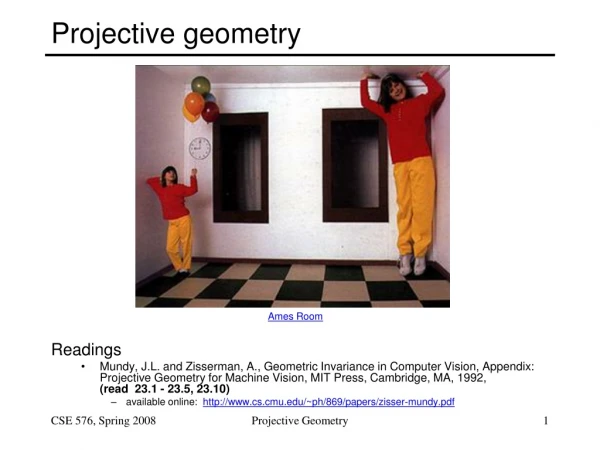
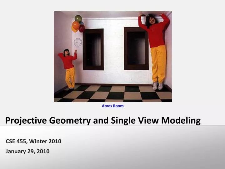
Ames Room. Projective Geometry and Single View Modeling. CSE 455, Winter 2010 January 29 , 2010. Announcements. Project 1a grades out https://catalysttools.washington.edu/gradebook/iansimon/17677 Statistics Mean 82.24 Median 86 Std. Dev. 17.88. Project 1a Common Errors.

E N D
Ames Room Projective Geometry and Single View Modeling CSE 455, Winter 2010 January 29, 2010
Announcements • Project 1a grades out • https://catalysttools.washington.edu/gradebook/iansimon/17677 • Statistics • Mean 82.24 • Median 86 • Std. Dev. 17.88
Project 1a Common Errors • Assuming odd size filters • Assuming square filters • Cross correlation vs. Convolution • Not normalizing the Gaussian filter • Resizing only works for shrinking not enlarging • Convolution operation is a cross-correlation where the filter is flipped both horizontally and vertically before being applied to the image:
Image rectification p’ p • To unwarp (rectify) an image • solve for homography H given p and p’ • solve equations of the form: wp’ = Hp • linear in unknowns: w and coefficients of H • H is defined up to an arbitrary scale factor • how many points are necessary to solve for H?
2n × 9 9 2n Solving for homographies A h 0 Defines a least squares problem: • Since h is only defined up to scale, solve for unit vector ĥ • Solution: ĥ = eigenvector of ATA with smallest eigenvalue • Works with 4 or more points
(x,y,1) image plane The projective plane • Why do we need homogeneous coordinates? • represent points at infinity, homographies, perspective projection, multi-view relationships • What is the geometric intuition? • a point in the image is a ray in projective space -y (sx,sy,s) (0,0,0) x -z • Each point(x,y) on the plane is represented by a ray(sx,sy,s) • all points on the ray are equivalent: (x, y, 1) (sx, sy, s)
A line is a plane of rays through origin • all rays (x,y,z) satisfying: ax + by + cz = 0 l p • A line is also represented as a homogeneous 3-vector l Projective lines • What does a line in the image correspond to in projective space?
vanishing point v Vanishing points image plane camera center C line on ground plane • Vanishing point • projection of a point at infinity
line on ground plane Vanishing points • Properties • Any two parallel lines have the same vanishing point v • The ray from C through v is parallel to the lines • An image may have more than one vanishing point • in fact every pixel is a potential vanishing point image plane vanishing point v camera center C line on ground plane
Today • Projective Geometry continued
Comparing heights Vanishing Point
Measuring height 5.4 5 Camera height 4 3.3 3 2.8 2 1 What is the height of the camera?
Least squares version • Better to use more than two lines and compute the “closest” point of intersection • See notes by Bob Collins for one good way of doing this: • http://www-2.cs.cmu.edu/~ph/869/www/notes/vanishing.txt Computing vanishing points (from lines) • Intersect p1q1 with p2q2 v q2 q1 p2 p1
Measuring height without a ruler Z C ground plane • Compute Z from image measurements • Need more than vanishing points to do this
The cross ratio • A Projective Invariant • Something that does not change under projective transformations (including perspective projection) The cross-ratio of 4 collinear points P4 P3 P2 P1 • Can permute the point ordering • 4! = 24 different orders (but only 6 distinct values) • This is the fundamental invariant of projective geometry
scene cross ratio t r C image cross ratio b vZ Measuring height T (top of object) R (reference point) H R B (bottom of object) ground plane scene points represented as image points as
Measuring height t v H image cross ratio vz r vanishing line (horizon) t0 vx vy H R b0 b
Measuring height v t1 b0 b1 vz r t0 vanishing line (horizon) t0 vx vy m0 b • What if the point on the ground plane b0 is not known? • Here the guy is standing on the box, height of box is known • Use one side of the box to help find b0 as shown above
Monocular Depth Cues • Stationary Cues: • Perspective • Relative size • Familiar size • Aerial perspective • Occlusion • Peripheral vision • Texture gradient
Camera calibration • Goal: estimate the camera parameters • Version 1: solve for projection matrix • Version 2: solve for camera parameters separately • intrinsics (focal length, principle point, pixel size) • extrinsics (rotation angles, translation) • radial distortion
= = similarly, π v , π v 2 Y 3 Z Vanishing points and projection matrix = vx (X vanishing point) Not So Fast! We only know v’s and o up to a scale factor • Need a bit more work to get these scale factors…
Finding the scale factors… • Let’s assume that the camera is reasonable • Square pixels • Image plane parallel to sensor plane • Principle point in the center of the image
Orthogonal vectors Solving for f Orthogonal vectors
Solving for a, b, and c Norm = 1/a Norm = 1/a • Solve for a, b, c • Divide the first two rows by f, now that it is known • Now just find the norms of the first three columns • Once we know a, b, and c, that also determines R • How about d? • Need a reference point in the scene
Solving for d • Suppose we have one reference height H • E.g., we known that (0, 0, H) gets mapped to (u, v) Finally, we can solve for t
Calibration using a reference object • Place a known object in the scene • identify correspondence between image and scene • compute mapping from scene to image • Issues • must know geometry very accurately • must know 3D->2D correspondence
Chromaglyphs Courtesy of Bruce Culbertson, HP Labs http://www.hpl.hp.com/personal/Bruce_Culbertson/ibr98/chromagl.htm
Estimating the projection matrix • Place a known object in the scene • identify correspondence between image and scene • compute mapping from scene to image
Direct linear calibration • Can solve for mij by linear least squares • use eigenvector trick that we used for homographies
Direct linear calibration • Advantage: • Very simple to formulate and solve • Disadvantages: • Doesn’t tell you the camera parameters • Doesn’t model radial distortion • Hard to impose constraints (e.g., known focal length) • Doesn’t minimize the right error function • For these reasons, nonlinear methods are preferred • Define error function E between projected 3D points and image positions • E is nonlinear function of intrinsics, extrinsics, radial distortion • Minimize E using nonlinear optimization techniques • e.g., variants of Newton’s method (e.g., Levenberg Marquart)
Alternative: multi-plane calibration Images courtesy Jean-Yves Bouguet, Intel Corp. • Advantage • Only requires a plane • Don’t have to know positions/orientations • Good code available online! • Intel’s OpenCV library:http://www.intel.com/research/mrl/research/opencv/ • Matlab version by Jean-Yves Bouget: http://www.vision.caltech.edu/bouguetj/calib_doc/index.html • Zhengyou Zhang’s web site: http://research.microsoft.com/~zhang/Calib/
Some Related Techniques • Image-Based Modeling and Photo Editing • Mok et al., SIGGRAPH 2001 • http://graphics.csail.mit.edu/ibedit/
Some Related Techniques • Single View Modeling of Free-Form Scenes • Zhang et al., CVPR 2001 • http://grail.cs.washington.edu/projects/svm/